It is possible to compute the low degree (co)homology of a finite group or monoid of small order directly from the bar resolution. The following commands take this approach to computing the fifth integral homology
H_5(Q_4, Z) = Z_2⊕ Z_2
of the quaternion group G=Q_4 of order 8.
gap> Q:=QuaternionGroup(8);;
gap> B:=BarComplexOfMonoid(Q,6);;
gap> C:=ContractedComplex(B);;
gap> Homology(C,5);
[ 2, 2 ]


gap> List([0..6],B!.dimension);
[ 1, 7, 49, 343, 2401, 16807, 117649 ]
gap> List([0..6],C!.dimension);
[ 1, 2, 2, 1, 2, 4, 102945 ]
However, this approach is of limited applicability since the bar resolution involves |G|^k free generators in degree k. A range of techniques, tailored to specific classes of groups, can be used to compute the (co)homology of larger finite groups.
This naive approach does have the merit of being applicable to arbitrary small monoids. The following calculates the homology in degrees ≤ 7 of a monoid of order 8, the monoid being specified by its multiplication table.
gap> T:=[ [  1,  1,  1,  4,  4,  4,  4,  1 ],
>         [  1,  1,  1,  4,  4,  4,  4,  2 ],
>         [  1,  1,  1,  4,  4,  4,  4,  3 ],
>         [  4,  4,  4,  1,  1,  1,  1,  4 ],
>         [  4,  4,  4,  1,  1,  1,  1,  5 ],
>         [  4,  4,  4,  1,  1,  1,  1,  6 ],
>         [  4,  4,  4,  1,  1,  1,  1,  7 ],
>         [  1,  2,  3,  4,  5,  6,  7,  8 ] ];;
gap> M:=MonoidByMultiplicationTable(T);
<monoid of size 8, with 8 generators>
gap> B:=BarComplexOfMonoid(M,8);;
gap> C:=ContractedComplex(B);;
gap> List([0..7],i->Homology(C,i));
[ [ 0 ], [ 2 ], [  ], [ 2 ], [  ], [ 2 ], [  ], [ 2 ] ]


gap> List([0..8],B!.dimension);
[ 1, 7, 49, 343, 2401, 16807, 117649, 823543, 5764801 ]
gap> List([0..8],C!.dimension);
[ 1, 1, 1, 1, 1, 1, 1, 1, 5044201 ]
The following example computes the seventh integral homology
H_7(M_23, Z) = Z_16⊕ Z_15
and fourth integral cohomomogy
H^4(M_24, Z) = Z_12
and fifth integral homology
H_5(M_24, Z) = Z_14
of the Mathieu groups M_23 and M_24. (Warning: the computation of H_7(M_23, Z) takes a couple of hours to run and the computation for H_5(M_24, Z) takes an hour to run.)
gap> GroupHomology(MathieuGroup(23),7);
[ 16, 3, 5 ]

gap> GroupCohomology(MathieuGroup(24),4);
[ 4, 3 ]

gap> GroupHomology(MathieuGroup(24),5);
[ 2, 7 ]
The following example computes the cokernel
coker( H_3(A_7, Z) → H_3(S_10, Z)) ≅ Z_2⊕ Z_2
of the degree-3 integral homomogy homomorphism induced by the canonical inclusion A_7 → S_10 of the alternating group on 7 letters into the symmetric group on 10 letters. The analogous cokernel with Z_2 homology coefficients is also computed.
gap> G:=SymmetricGroup(10);;
gap> H:=AlternatingGroup(7);;
gap> f:=GroupHomomorphismByFunction(H,G,x->x);;
gap> F:=GroupHomology(f,3);
MappingByFunction( Pcp-group with orders [ 4, 3 ], Pcp-group with orders
[ 2, 2, 4, 3 ], function( x ) ... end )
gap> AbelianInvariants(Range(F)/Image(F));
[ 2, 2 ]

gap> Fmod2:=GroupHomology(f,3,2);;
gap> AbelianInvariants(Range(Fmod2)/Image(Fmod2));
[ 2, 2 ]
The following example computes the third integral homology of the Weyl group W=Weyl(E_8), a group of order 696729600.
H_3(Weyl(E_8), Z) = Z_2 ⊕ Z_2 ⊕ Z_12
gap> L:=SimpleLieAlgebra("E",8,Rationals);;
gap> W:=WeylGroup(RootSystem(L));;
gap> Order(W);
696729600
gap> GroupHomology(W,3);
[ 2, 2, 4, 3 ]
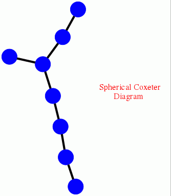
The preceding calculation could be achieved more quickly by noting that W=Weyl(E_8) is a Coxeter group, and by using the associated Coxeter polytope. The following example uses this approach to compute the fourth integral homology of W. It begins by displaying the Coxeter diagram of W, and then computes
H_4(Weyl(E_8), Z) = Z_2 ⊕ Z_2 ⊕ Z_2 ⊕ Z_2.
gap> D:=[[1,[2,3]],[2,[3,3]],[3,[4,3],[5,3]],[5,[6,3]],[6,[7,3]],[7,[8,3]]];;
gap> CoxeterDiagramDisplay(D);
gap> polytope:=CoxeterComplex_alt(D,5);;
gap> R:=FreeGResolution(polytope,5);
Resolution of length 5 in characteristic 0 for <matrix group with
8 generators> .
No contracting homotopy available.

gap> C:=TensorWithIntegers(R);
Chain complex of length 5 in characteristic 0 .

gap> Homology(C,4);
[ 2, 2, 2, 2 ]
The following example computes the sixth mod-2 homology of the Sylow 2-subgroup Syl_2(M_24) of the Mathieu group M_24.
H_6(Syl_2(M_24), Z_2) = Z_2^143
gap> GroupHomology(SylowSubgroup(MathieuGroup(24),2),6,2);
[ 2, 2, 2, 2, 2, 2, 2, 2, 2, 2, 2, 2, 2, 2, 2, 2, 2, 2, 2, 2, 2, 2,
  2, 2, 2, 2, 2, 2, 2, 2, 2, 2, 2, 2, 2, 2, 2, 2, 2, 2, 2, 2, 2, 2,
  2, 2, 2, 2, 2, 2, 2, 2, 2, 2, 2, 2, 2, 2, 2, 2, 2, 2, 2, 2, 2, 2,
  2, 2, 2, 2, 2, 2, 2, 2, 2, 2, 2, 2, 2, 2, 2, 2, 2, 2, 2, 2, 2, 2,
  2, 2, 2, 2, 2, 2, 2, 2, 2, 2, 2, 2, 2, 2, 2, 2, 2, 2, 2, 2, 2, 2,
  2, 2, 2, 2, 2, 2, 2, 2, 2, 2, 2, 2, 2, 2, 2, 2, 2, 2, 2, 2, 2, 2,
  2, 2, 2, 2, 2, 2, 2, 2, 2, 2, 2 ]
The following example computes the sixth mod-2 homology of the Unitary group U_3(4) of order 312000.
H_6(U_3(4), Z_2) = Z_2^4
gap> G:=GU(3,4);;
gap> Order(G);
312000
gap> GroupHomology(G,6,2);
[ 2, 2, 2, 2 ]
The following example constructs the Poincare series
p(x)=frac1-x^3+3*x^2-3*x+1
for the cohomology H^∗(Syl_2(M_12, F_2). The coefficient of x^n in the expansion of p(x) is equal to the dimension of the vector space H^n(Syl_2(M_12, F_2). The computation involves Singular's Groebner basis algorithms and the Lyndon-Hochschild-Serre spectral sequence.
gap> G:=SylowSubgroup(MathieuGroup(12),2);;
gap> P:=PoincareSeriesLHS(G);
(1)/(-x_1^3+3*x_1^2-3*x_1+1)
The additional following command uses the Poincare series
gap> RankHomologyPGroup(G,P,1000);
251000
to determine that H_1000(Syl_2(M_12, Z) is a direct sum of 251000 non-trivial cyclic 2-groups.
The following example constructs the series
p(x)=fracx^4-x^3+x^2-x+1x^6-x^5+x^4-2*x^3+x^2-x+1
whose coefficient of x^n is equal to the dimension of the vector space H^n(M_11, F_2) for all n in the range 0≤ n≤ 14. The coefficient is not guaranteed correct for n≥ 15.
gap> PoincareSeriesPrimePart(MathieuGroup(11),2,14);
(x_1^4-x_1^3+x_1^2-x_1+1)/(x_1^6-x_1^5+x_1^4-2*x_1^3+x_1^2-x_1+1)
The following example computes
H_4(N, Z) = (Z_3)^4 ⊕ Z^84
for the free nilpotent group N of class 2 on four generators.
gap> F:=FreeGroup(4);; N:=NilpotentQuotient(F,2);;
gap> GroupHomology(N,4);
[ 3, 3, 3, 3, 0, 0, 0, 0, 0, 0, 0, 0, 0, 0, 0, 0, 0, 0, 0, 0, 0, 0,
  0, 0, 0, 0, 0, 0, 0, 0, 0, 0, 0, 0, 0, 0, 0, 0, 0, 0, 0, 0, 0, 0,
  0, 0, 0, 0, 0, 0, 0, 0, 0, 0, 0, 0, 0, 0, 0, 0, 0, 0, 0, 0, 0, 0,
  0, 0, 0, 0, 0, 0, 0, 0, 0, 0, 0, 0, 0, 0, 0, 0, 0, 0, 0, 0, 0, 0 ]
The following example computes
H_5(G, Z) = Z_2 ⊕ Z_2
for the 3-dimensional crystallographic space group G with Hermann-Mauguin symbol "P62"
gap> GroupHomology(SpaceGroupBBNWZ("P62"),5);
[ 2, 2 ]
The following example computes
H^5(G, Z)= Z
for an almost crystallographic group.
gap> G:=AlmostCrystallographicPcpGroup( 4, 50, [ 1, -4, 1, 2 ] );;
gap> GroupCohomology(G,4);
[ 0 ]
The following example computes
H_6(SL_2(cal O), Z) = Z_2 ⊕ Z_12
for cal O the ring of integers of the number field Q(sqrt-2).
gap> C:=ContractibleGcomplex("SL(2,O-2)");;
gap> R:=FreeGResolution(C,7);;
gap> Homology(TensorWithIntegers(R),6);
[ 2, 12 ]
The following example computes
H_n(SL_4( Z), Z) = { beginarrayll 0, &n=1 Z_2 ⊕ Z_2, & n=2 Z ⊕ Z_2 ⊕ Z_12 ⊕ Z_240, &n=3 Z_2 ⊕ Z_2 ⊕ Z_10, & n=4 ( Z_2)^7, & n=5 . endarray.
gap> K:=ContractibleGcomplex("SL4Z_d");;
gap> R:=FreeGResolution(K,6);;
gap> Homology(TensorWithIntegers(R),1);
[  ]
gap> Homology(TensorWithIntegers(R),2);
[ 2, 2 ]
gap> Homology(TensorWithIntegers(R),3);
[ 2, 12, 240, 0 ]
gap> Homology(TensorWithIntegers(R),4);
[ 2, 2, 10 ]
gap> Homology(TensorWithIntegers(R),5);
[ 2, 2, 2, 2, 2, 2, 2 ]
For the congruence subgroup Γ_0(101) < SL_3( Z) the following example computes
H_n(Γ_0(101), Z)= {beginarrayll Z_100, & n=1 ( Z_2)^15⊕ ( Z_4)^4, &n=2 ( Z_4)^2 ⊕ ( Z_12)^2 ⊕ Z^16, & n=3 . endarray.
gap> G:=HAPCongruenceSubgroupGamma0(3,101);;
gap> K:=ContractibleGcomplex("SL(3,Z)a");;
gap> R:=FreeGResolution(K,4);;
gap> S:=ResolutionFiniteSubgroup(R,G);;
gap> C:=TensorWithIntegers(S);;
gap> D:=ContractedComplex(C);;
gap> Homology(D,1);
[ 100 ]
gap> Homology(D,2);
[ 2, 2, 2, 2, 2, 2, 2, 2, 2, 2, 2, 2, 2, 2, 2, 4, 4, 4, 4 ]
gap> Homology(D,3);
[ 4, 4, 12, 12, 0, 0, 0, 0, 0, 0, 0, 0, 0, 0, 0, 0, 0, 0, 0, 0 ]
In the preceding code K is a representation of a 3-dimensional contractible regular CW-complex (a 'well-rounded retract') on which SL_3( Z) acts by permuting cells and for which every cell stabilizer is a finite group. The following code shows that there is just one orbit of 3-cells and displays the 1-skeleton of the closure of a 3-cell. (Further investigation of K shows that the 2-cells are either hexagonal or triangular. Each hexagonal 2-cell is incident with three 3-cells; each triangular 2-cell is incident with four 3-cells.)
gap> K:=ContractibleGcomplex("SL(3,Z)a");;
gap> List([0..4],K!.dimension);
[ 1, 1, 2, 1, 0 ]
gap> Y:=GComplexToFiniteRegularCWRegion(K,0);;
gap> Display(GraphOfRegularCWComplex(Y));
The command Y:=GComplexToFiniteRegularCWRegion(K,r) returns a 'ball of radius r' in the contractible CW-complex represented by K for any integer r≥ 0. The ball is returned as a finite regular CW-complex. For instance, the following code constructs a ball of radius r=7 and builds a contracting disctete vector field on this ball. The component Y!.G_Cells[n+1][k] returns a pair [e,g] with integer e specifying a representative of an orbit of n-cells in K and g an element in SL(3, Z) such that the kth n-cell of Y corresponds to g.e .
gap> K:=ContractibleGcomplex("SL(3,Z)a");;
gap> Y:=GComplexToFiniteRegularCWRegion(K,7);;
gap> Size(Y); #number of cells in Y
90537003
gap> Y!.nrCells(3); #number of 3-cells in Y
4729285
gap> CriticalCells(Y);
[ [ 0, 18456062 ] ]
The following example computes
H_n(G, Z) ={ beginarrayll Z &n=0,1,7,8 Z_2, &n=2,3 Z_2⊕ Z_6, &n=4,6 Z_3 ⊕ Z_6,& n=5 0, &n>8 endarray.
for G the Artin group of type E_8. (Similar commands can be used to compute a resolution and homology of arbitrary Artin monoids and, in thoses cases such as the spherical cases where the K(π,1)-conjecture is known to hold, the homology is equal to that of the corresponding Artin group.)
gap> D:=[[1,[2,3]],[2,[3,3]],[3,[4,3],[5,3]],[5,[6,3]],[6,[7,3]],[7,[8,3]]];;
gap> CoxeterDiagramDisplay(D);;
gap> R:=ResolutionArtinGroup(D,9);;
gap> C:=TensorWithIntegers(R);;
gap> List([0..8],n->Homology(C,n));
[ [ 0 ], [ 0 ], [ 2 ], [ 2 ], [ 2, 6 ], [ 3, 6 ], [ 2, 6 ], [ 0 ], [ 0 ] ]
The Artin group G projects onto the Coxeter group W of type E_8. The group W has a natural representation as a group of 8× 8 integer matrices. This projection gives rise to a representation ρ: G→ GL_8( Z). The following command computes the cohomology group H^6(G,ρ) = ( Z_2)^6.
gap> G:=R!.group;;
gap> gensG:=GeneratorsOfGroup(G);;
gap> W:=CoxeterDiagramMatCoxeterGroup(D);;
gap> gensW:=GeneratorsOfGroup(W);;
gap> rho:=GroupHomomorphismByImages(G,W,gensG,gensW);;
gap> C:=HomToIntegralModule(R,rho);;
gap> Cohomology(C,6);
[ 2, 2, 2, 2, 2, 2 ]
The following example computes
H_5(G, Z) = Z_2⊕ Z_2⊕ Z_2 ⊕ Z_2 ⊕ Z_2
for G the graph of groups corresponding to the amalgamated product G=S_5*_S_3S_4 of the symmetric groups S_5 and S_4 over the canonical subgroup S_3.
gap> S5:=SymmetricGroup(5);SetName(S5,"S5");
gap> S4:=SymmetricGroup(4);SetName(S4,"S4");
gap> A:=SymmetricGroup(3);SetName(A,"S3");
gap> AS5:=GroupHomomorphismByFunction(A,S5,x->x);
gap> AS4:=GroupHomomorphismByFunction(A,S4,x->x);
gap> D:=[S5,S4,[AS5,AS4]];
gap> GraphOfGroupsDisplay(D);
gap> R:=ResolutionGraphOfGroups(D,6);;
gap> Homology(TensorWithIntegers(R),5);
[ 2, 2, 2, 2, 2 ]
The next example computes the integral homology of SL_2( Z) in degrees ≤ 5 using the isomorphism SL_2( Z) ≅ C_4∗_C_2C_6.
gap> x:=(1,2,3,4,5,6,7,8,9,10,11,12);;
gap> C6:=Group(x^2);;SetName(C6,"C6");;
gap> C4:=Group(x^3);;SetName(C4,"C4");;
gap> C2:=Group(x^6);;SetName(C2,"C2");;
gap> C2C6:=GroupHomomorphismByFunction(C2,C6,x->x);;
gap> C2C4:=GroupHomomorphismByFunction(C2,C4,x->x);;
gap> D:=[C6,C4,[C2C6,C2C4]];;
gap> GraphOfGroupsDisplay(D);
gap> R:=ResolutionGraphOfGroups(D,6);;
gap> List([0..5],n->Homology(TensorWithIntegers(R),n));
[ [ 0 ], [ 12 ], [  ], [ 12 ], [  ], [ 12 ] ]
The next commands compute the integral homology in degree 7 of a graph of groups corresponding to the HNN extension G=H*_A where H is the symmetric group H=S_5 and A is the subgroup A=S_3 and f:A→ H is the homomorphism (1,2) → (3,4), (1,2,3) → (3,4,5). The HNN extension G is obtained from H by adding a generator t subject to the relations t^-1 a t = f(a) for a ∈ A.
gap> S5:=SymmetricGroup(5);SetName(S5,"S5");;
gap> A:=SymmetricGroup(3);SetName(A,"S3");;
gap> f:=GroupHomomorphismByImages(A,S5,[(1,2),(1,2,3)],[(3,4),(3,4,5)]);;
gap> g:=GroupHomomorphismByFunction(A,S5,x->x);;
gap> D:=[S5,[f,g]];;
gap> GraphOfGroupsDisplay(D);;

gap> R:=ResolutionGraphOfGroups(D,8);;
gap> Homology(TensorWithIntegers(R),7);
[ 2, 2, 60 ]
One method of producting a Lie algebra L from a group G is by forming the direct sum L(G) = G/γ_2G ⊕ γ_2G/γ_3G ⊕ γ_3G/γ_4G ⊕ ⋯ of the quotients of the lower central series γ_1G=G, γ_n+1G=[γ_nG,G]. Commutation in G induces a Lie bracket L(G)× L(G) → L(G).
The homology H_n(L) of a Lie algebra (with trivial coefficients) can be calculated as the homology of the Chevalley-Eilenberg chain complex C_∗(L). This chain complex is implemented in HAP in the cases where the underlying additive group of L is either finitely generated torsion free or finitely generated of prime exponent p. In these two cases the ground ring for the Lie algebra/ Chevalley-Eilenberg complex is taken to be Z and Z_p respectively.
For example, consider the quotient G=F/γ_8F of the free group F=F(x,y) on two generators by eighth term of its lower central series. So G is the free nilpotent group of class 7 on two generators. The following commands compute H_4(L(G)) = Z_2^77 ⊕ Z_6^8 ⊕ Z_12^51 ⊕ Z_132^11 ⊕ Z^2024 and show that the fourth homology in this case contains 2-, 3- and 11-torsion. (The commands take an hour or so to complete.)
gap> G:=Image(NqEpimorphismNilpotentQuotient(FreeGroup(2),7));;
gap> L:=LowerCentralSeriesLieAlgebra(G);;
gap> h:=LieAlgebraHomology(L,4);;
gap> Collected(h);
[ [ 0, 2024 ], [ 2, 77 ], [ 6, 8 ], [ 12, 51 ], [ 132, 11 ] ]
For a free nilpotent group G the additive homology H_n(L(G)) of the Lie algebra can be computed more quickly in HAP than the integral group homology H_n(G, Z). Clearly there are isomorphismsH_1(G) ≅ H_1(L(G)) ≅ G_ab of abelian groups in homological degree n=1. Hopf's formula can be used to establish an isomorphism H_2(G) ≅ H_2(L(G)) also in degree n=2. The following two theorems provide further isomorphisms that allow for the homology of a free nilpotent group to be calculated more efficiently as the homology of the associated Lie algebra.
Theorem 1. [KS98] Let G be a finitely generated free nilpotent group of class 2. Then the integral group homology H_n(G, Z) is isomorphic to the integral Lie algebra homology H_n(L(G), Z) in each degree n≥0.
Theorem 2. [IO01] Let G be a finitely generated free nilpotent group (of any class). Then the integral group homology H_n(G, Z) is isomorphic to the integral Lie algebra homology H_n(L(G), Z) in degrees n=0, 1, 2, 3.
We should remark that experimentation on free nilpotent groups of class ≥ 4 has not yielded a group for which the isomorphism H_n(G, Z) ≅ H_n(L(G), G) fails. For instance, the isomorphism holds in degree n=4 for the free nilpotent group of class 5 on two generators, and for the free nilpotent group of class 2 on four generators:
gap> G:=Image(NqEpimorphismNilpotentQuotient(FreeGroup(2),5));;
gap> L:=LowerCentralSeriesLieAlgebra(G);;
gap> Collected( LieAlgebraHomology(L,4) );
[ [ 0, 85 ], [ 7, 1 ] ]
gap> Collected( GroupHomology(G,4) );
[ [ 0, 85 ], [ 7, 1 ] ]

gap> G:=Image(NqEpimorphismNilpotentQuotient(FreeGroup(4),2));;
gap> L:=LowerCentralSeriesLieAlgebra(G);;
gap> Collected( LieAlgebraHomology(L,4) );
[ [ 0, 84 ], [ 3, 4 ] ]
gap> Collected( GroupHomology(G,4) );
[ [ 0, 84 ], [ 3, 4 ] ]
There are various ways to represent a ZG-module A with action G× A → A, (g,a)↦ α(g,a).
One possibility is to use the data type of a G-Outer Group which involves three components: an ActedGroup A; an Acting Group G; a Mapping (g,a)↦ α(g,a). The following example uses this data type to compute the cohomology H^4(G,A) = Z_5 ⊕ Z_10 of the symmetric group G=S_6 with coefficients in the integers A= Z where odd permutations act non-trivially on A.
gap> G:=SymmetricGroup(6);;

gap> A:=AbelianPcpGroup([0]);;
gap> alpha:=function(g,a); return a^SignPerm(g); end;;
gap> A:=GModuleAsGOuterGroup(G,A,alpha);
ZG-module with abelian invariants [ 0 ] and G= SymmetricGroup( [ 1 .. 6 ] )

gap> R:=ResolutionFiniteGroup(G,5);;
gap> C:=HomToGModule(R,A);
G-cocomplex of length 5 .

gap> Cohomology(C,4);
[ 2, 2, 5 ]
If A= Z^n and G acts as
G× A → A, (g, v) ↦ ρ(g) v
where ρ: G→ Gl_n( Z) is a (not necessarily faithful) matrix representation of degree n then we can avoid the use of G-outer groups and use just the homomorphism ρ instead. The following example uses this data type to compute the cohomology
H^6(G,A) = Z_2
and the homology
H_6(G,A) = 0
of the alternating group G=A_5 with coefficients in A= Z^5 where elements of G act on Z^5 via an irreducible representation.
gap> G:=AlternatingGroup(5);;
gap> rho:=IrreducibleRepresentations(G)[5];
[ (1,2,3,4,5), (3,4,5) ] ->
[
  [ [ 0, 0, 1, 0, 0 ], [ -1, -1, 0, 0, 1 ], [ 0, 1, 1, 1, 0 ],
      [ 1, 0, -1, 0, -1 ], [ -1, -1, 0, -1, 0 ] ],
  [ [ -1, -1, 0, 0, 1 ], [ 1, 0, -1, 0, -1 ], [ 0, 0, 0, 0, 1 ],
      [ 0, 0, 1, 0, 0 ], [ 0, 0, 0, 1, 0 ] ] ]
gap> R:=ResolutionFiniteGroup(G,7);;
gap> C:=HomToIntegralModule(R,rho);;
gap> Cohomology(C,6);
[ 2 ]
gap> D:=TensorWithIntegralModule(R,rho);
Chain complex of length 7 in characteristic 0 .

gap> Homology(D,6);
[  ]
If V=K^d is a vetor space of dimension d over the field K=GF(p) with p a prime and G acts on V via a homomorphism ρ: G→ GL_d(K) then the homology H^n(G,V) can again be computed without the use of G-outer groups. As an example, the following commands compute
H^4(GL(3,2),V) =K^2
where K=GF(2) and GL(3,2) acts with its natural action on V=K^3.
gap> G:=GL(3,2);;
gap> rho:=GroupHomomorphismByFunction(G,G,x->x);;
gap> R:=ResolutionFiniteGroup(G,5);;
gap> C:=HomToModPModule(R,rho);;
gap> Cohomology(C,4);
2
The following example constructs the Artin braid group G=B_3 on three strings, the surjection G↠ S_3, a complex representation S_3→ GL_2( C) and the composite representation ρ: G→ GL_2( C). The group G acts on the vector space V= C⊕ C via ρ. Then the dimensions of the cohomology groups H^n(G,V) are computed.
gap> D:=[[1,[2,3]],[2,[3,3]]];;
gap> R:=ResolutionArtinGroup(D,4);;
gap> G:=R!.group;; #Braid group
gap> r:=[G.1^2,G.2^2,G.3^2];;Q:=G/r;;
gap> q:=GroupHomomorphismByImages(G,Q,GeneratorsOfGroup(G),GeneratorsOfGroup(Q));;
gap> h:=IrreducibleRepresentations(Q)[3];
Pcgs([ f1^-1*f2^-1*f3^-2*f1^-1, f3^-1*f2^-1*f1^-1*f2^-1, f2*f3^-1*f1^-1*f2^-1,
  f3^-1*f1^-1 ]) -> [ [ [ 0, 1 ], [ 1, 0 ] ], [ [ E(3), 0 ], [ 0, E(3)^2 ] ],
  [ [ 1, 0 ], [ 0, 1 ] ], [ [ 1, 0 ], [ 0, 1 ] ] ]
gap> rho:=GroupHomomorphismByFunction(G,Image(h),x->Image(h,Image(q,x)));;
gap> C:=HomToModuleOverCyclotomicField(R,rho);
Cochain complex of length 4 over field of characteristic 0.

gap> Cohomology(C,1);
1
gap> Cohomology(C,2);
1
It can be computationally difficult to compute resolutions for large finite groups. But the p-primary part of the homology can be computed using resolutions of Sylow p-subgroups. This approach is used in the following example that computes the 2-primary part
H_2(G, Z)_(2) = Z_2 ⊕ Z_2⊕ Z_2
of the degree 2 integral homology of the Rubik's cube group G. This group has order 43252003274489856000.
gap> gens:= [
>    ( 1, 3, 8, 6)( 2, 5, 7, 4)( 9,33,25,17)(10,34,26,18)(11,35,27,19),
>    ( 9,11,16,14)(10,13,15,12)( 1,17,41,40)( 4,20,44,37)( 6,22,46,35),
>    (17,19,24,22)(18,21,23,20)( 6,25,43,16)( 7,28,42,13)( 8,30,41,11),
>    (25,27,32,30)(26,29,31,28)( 3,38,43,19)( 5,36,45,21)( 8,33,48,24),
>    (33,35,40,38)(34,37,39,36)( 3, 9,46,32)( 2,12,47,29)( 1,14,48,27),
>    (41,43,48,46)(42,45,47,44)(14,22,30,38)(15,23,31,39)(16,24,32,40)
>  ];; G:=Group(gens);;P:=SylowSubgroup(G,2);;
gap> R:=ResolutionNormalSeries(BigStepUCS(P,6),3);;
gap> PrimePartDerivedFunctorViaSubgroupChain(G,R,TensorWithIntegers,2);
[ 2, 2, 2 ]
The same approach is used in the following example that computes the 2-primary part
H_11(A_7,A)_(2) = Z_2 ⊕ Z_2⊕ Z_4
of the degree 11 homology of the alternating group A_7 of degree 7 with coefficients in the module A= Z^7 on which A_7 acts by permuting basis vectors.
gap> G:=AlternatingGroup(7);;
gap> rho:=PermToMatrixGroup(G);;
gap> R:=ResolutionFiniteGroup(SylowSubgroup(G,2),12);;
gap> F:=function(X); return TensorWithIntegralModule(X,rho); end;;
gap> PrimePartDerivedFunctorViaSubgroupChain(G,R,F,11);
[ 2, 2, 4 ]
Similar commands compute
H_3(A_10,A)_(2) = Z_4
with coefficient module A= Z^10 on which A_10 acts by permuting basis vectors.
gap> G:=AlternatingGroup(10);;
gap> rho:=PermToMatrixGroup(G);;
gap> R:=ResolutionFiniteGroup(SylowSubgroup(G,2),4);;
gap> F:=function(X); return TensorWithIntegralModule(X,rho); end;;
gap> PrimePartDerivedFunctorViaSubgroupChain(G,R,F,3);
[ 4 ]
The following commands compute
H_100(GL(3,2),V)= K^34
where V is the vector space of dimension 3 over K=GF(2) acting via some irreducible representation ρ: GL(3,2) → GL(V).
gap> G:=GL(3,2);;
gap> rho:=IrreducibleRepresentations(G,GF(2))[3];
CompositionMapping( [ (5,7)(6,8), (2,3,5)(4,7,6) ] ->
[ <an immutable 3x3 matrix over GF2>, <an immutable 3x3 matrix over GF2> ],
 <action isomorphism> )
gap> F:=function(X); return TensorWithModPModule(X,rho); end;;
gap> S:=ResolutionPrimePowerGroup(SylowSubgroup(G,2),101);;
gap> PrimePartDerivedFunctorViaSubgroupChain(G,S,F,100);
[ 2, 2, 2, 2, 2, 2, 2, 2, 2, 2, 2, 2, 2, 2, 2, 2, 2, 2, 2, 2, 2, 2, 2, 2, 2,
  2, 2, 2, 2, 2, 2, 2, 2, 2 ]
Suppose given a group homomorphism f: G_1→ G_2 and a G_2-module A. Then A is naturally a G_1-module with action via f, and there is an induced cohomology homomorphism H^n(f,A): H^n(G_2,A) → H^n(G_1,A).
The following example computes this cohomology homomorphism in degree n=6 for the inclusion f: A_5 → S_5 and A= Z^5 with action that permutes the canonical basis. The final commands determine that the kernel of the homomorphism H^6(f,A) is the Klein group of order 4 and that the cokernel is cyclic of order 6.
gap> G1:=AlternatingGroup(5);;
gap> G2:=SymmetricGroup(5);;
gap> f:=GroupHomomorphismByFunction(G1,G2,x->x);;
gap> pi:=PermToMatrixGroup(G2,5);;
gap> R1:=ResolutionFiniteGroup(G1,7);;
gap> R2:=ResolutionFiniteGroup(G2,7);;
gap> F:=EquivariantChainMap(R1,R2,f);;
gap> C:=HomToIntegralModule(F,pi);;
gap> c:=Cohomology(C,6);
[ g1, g2, g3 ] -> [ id, id, g3 ]

gap> AbelianInvariants(Kernel(c));
[ 2, 2 ]
gap> AbelianInvariants(Range(c)/Image(c));
[ 2, 3 ]
A short exact sequence of ZG-modules A ↣ B ↠ C induces a long exact sequence of cohomology groups
→ H^n(G,A) → H^n(G,B) → H^n(G,C) → H^n+1(G,A) → .
Consider the symmetric group G=S_4 and the sequence Z_4 ↣ Z_8 ↠ Z_2 of trivial ZG-modules. The following commands compute the induced cohomology homomorphism
f: H^3(S_4, Z_4) → H^3(S_4, Z_8)
and determine that the image of this induced homomorphism has order 8 and that its kernel has order 2.
gap> G:=SymmetricGroup(4);;
gap> x:=(1,2,3,4,5,6,7,8);;
gap> a:=Group(x^2);;
gap> b:=Group(x);;
gap> ahomb:=GroupHomomorphismByFunction(a,b,y->y);;
gap> A:=TrivialGModuleAsGOuterGroup(G,a);;
gap> B:=TrivialGModuleAsGOuterGroup(G,b);;
gap> phi:=GOuterGroupHomomorphism();;
gap> phi!.Source:=A;;
gap> phi!.Target:=B;;
gap> phi!.Mapping:=ahomb;;

gap> Hphi:=CohomologyHomomorphism(phi,3);;

gap> Size(ImageOfGOuterGroupHomomorphism(Hphi));
8

gap> Size(KernelOfGOuterGroupHomomorphism(Hphi));
2
The following commands then compute the homomorphism
H^3(S_4, Z_8) → H^3(S_4, Z_2)
induced by Z_4 ↣ Z_8 ↠ Z_2, and determine that the kernel of this homomorphsim has order 8.
gap> bhomc:=NaturalHomomorphismByNormalSubgroup(b,a);
gap> B:=TrivialGModuleAsGOuterGroup(G,b);
gap> C:=TrivialGModuleAsGOuterGroup(G,Image(bhomc));
gap> psi:=GOuterGroupHomomorphism();
gap> psi!.Source:=B;
gap> psi!.Target:=C;
gap> psi!.Mapping:=bhomc;

gap> Hpsi:=CohomologyHomomorphism(psi,3);

gap> Size(KernelOfGOuterGroupHomomorphism(Hpsi));
8
The following commands then compute the connecting homomorphism
H^2(S_4, Z_2) → H^3(S_4, Z_4)
and determine that the image of this homomorphism has order 2.
gap> delta:=ConnectingCohomologyHomomorphism(psi,2);;
gap> Size(ImageOfGOuterGroupHomomorphism(delta));
Note that the various orders are consistent with exactness of the sequence
H^2(S_4, Z_2) → H^3(S_4, Z_4) → H^3(S_4, Z_8) → H^3(S_4, Z_2) .
Consider the action of the symmetric group G=S_5 on A= Z^5 which permutes the canonical basis. The action restricts to the sylow 2-subgroup P=Syl_2(G). The following commands compute the cohomology transfer homomorphism t^4: H^4(P,A) → H^4(S_5,A) and determine its kernel and image. The integral homology transfer t_4: H_4(S_5, Z) → H_5(P, Z) is also computed.
gap> G:=SymmetricGroup(5);;
gap> P:=SylowSubgroup(G,2);;
gap> R:=ResolutionFiniteGroup(G,5);;
gap> A:=PermToMatrixGroup(G);;
gap> tr:=TransferCochainMap(R,P,A);
Cochain Map between complexes of length 5 .

gap> t4:=Cohomology(tr,4);
[ g1, g2, g3, g4 ] -> [ id, g1, g2, g4 ]
gap> StructureDescription(Kernel(t4));
"C2 x C2"
gap> StructureDescription(Image(t4));
"C4 x C2"

gap> tr:=TransferChainMap(R,P);
Chain Map between complexes of length 5 .

gap> Homology(tr,4);
[ g1 ] -> [ g1 ]
A spherical 3-manifold is a 3-manifold arising as the quotient S^3/Γ of the 3-sphere S^3 by a finite subgroup Γ of SO(4) acting freely as rotations. The geometrization conjecture, proved by Grigori Perelman, implies that every closed connected 3-manifold with a finite fundamental group is homeomorphic to a spherical 3-manifold.
A spherical 3-manifold S^3/Γ has finite fundamental group isomorphic to Γ. This fundamental group is one of:
Γ=C_m=⟨ x | x^m⟩ (cyclic fundamental group)
Γ=C_m× ⟨ x,y | xyx^-1=y^-1, x^2^k=y^n ⟩ for integers k, m≥ 1, n≥ 2 and m coprime to 2n (prism manifold case)
Γ= C_m× ⟨ x,y, z | (xy)^2=x^2=y^2, zxz^-1=y, zyz^-1=xy, z^3^k=1⟩ for integers k,m≥ 1 and m coprime to 6 (tetrahedral case)
Γ=C_m×⟨ x,y | (xy)^2=x^3=y^4⟩ for m≥ 1 coprime to 6 (octahedral case)
Γ=C_m× ⟨ x,y | (xy)^2=x^3=y^5⟩ for m≥ 1 coprime to 30 (icosahedral case).
This list of cases is taken from the Wikipedia pages. The group Γ has periodic cohomology since it acts on a sphere. The cyclic group has period 2 and in the other four cases it has period 4. (Recall that in general a finite group G has periodic cohomology of period n if there is an element u∈ H^n(G, Z) such that the cup product - ∪ u: H^k(G, Z) → H^k+n(G, Z) is an isomorphism for all k≥ 1. It can be shown that G has periodic cohomology of period n if and only if H^n(G, Z)= Z_|G|.)
The cohomology of the cyclic group is well-known, and the cohomology of a direct product can be obtained from that of the factors using the Kunneth formula.
In the icosahedral case with m=1 the following commands yield $$H^\ast(\Gamma,\mathbb Z)=Z[t]/(120t=0)$$ with generator t of degree 4. The final command demonstrates that a periodic resolution is used in the computation.
gap> F:=FreeGroup(2);;x:=F.1;;y:=F.2;;
gap> G:=F/[(x*y)^2*x^-3, x^3*y^-5];;
gap> Order(G);
120
gap> R:=ResolutionSmallGroup(G,5);;
gap> n:=0;;Cohomology(HomToIntegers(R),n);
[ 0 ]
gap> n:=1;;Cohomology(HomToIntegers(R),n);
[  ]
gap> n:=2;;Cohomology(HomToIntegers(R),n);
[  ]
gap> n:=3;;Cohomology(HomToIntegers(R),n);
[  ]
gap> n:=4;;Cohomology(HomToIntegers(R),n);
[ 120 ]

gap> List([0..5],k->R!.dimension(k));
[ 1, 2, 2, 1, 1, 2 ]
In the octahedral case with m=1 we obtain $$H^\ast(\Gamma,\mathbb Z) = \mathbb Z[s,t]/(s^2=24t, 2s=0, 48t=0)$$ where s has degree 2 and t has degree 4, from the following commands.
gap> F:=FreeGroup(2);;x:=F.1;;y:=F.2;;
gap> G:=F/[(x*y)^2*x^-3, x^3*y^-4];;
gap> Order(G);
48
gap> R:=ResolutionFiniteGroup(G,5);;
gap> n:=0;;Cohomology(HomToIntegers(R),n);
[ 0 ]
gap> n:=1;;Cohomology(HomToIntegers(R),n);
[  ]
gap> n:=2;;Cohomology(HomToIntegers(R),n);
[ 2 ]
gap> n:=3;;Cohomology(HomToIntegers(R),n);
[  ]
gap> n:=4;;Cohomology(HomToIntegers(R),n);
[ 48 ]
gap> IntegralCupProduct(R,[1],[1],2,2);
[ 24 ]
In the tetrahedral case with m=1 we obtain $$H^\ast(\Gamma,\mathbb Z) = \mathbb Z[s,t]/(s^2=16t, 3s=0, 24t=0)$$ where s has degree 2 and t has degree 4, from the following commands.
gap> F:=FreeGroup(3);;x:=F.1;;y:=F.2;;z:=F.3;;
gap> G:=F/[(x*y)^2*x^-2, x^2*y^-2, z*x*z^-1*y^-1, z*y*z^-1*y^-1*x^-1,z^3];;
gap> Order(G);
24
gap> R:=ResolutionFiniteGroup(G,5);;
gap> n:=1;;Cohomology(HomToIntegers(R),n);
[  ]
gap> n:=2;;Cohomology(HomToIntegers(R),n);
[ 3 ]
gap> n:=3;;Cohomology(HomToIntegers(R),n);
[  ]
gap> n:=4;;Cohomology(HomToIntegers(R),n);
[ 24 ]
gap> IntegralCupProduct(R,[1],[1],2,2);
[ 16 ]
A theoretical calculation of the integral and mod-p cohomology rings of all of these fundamental groups of spherical 3-manifolds is given in [TZ08].
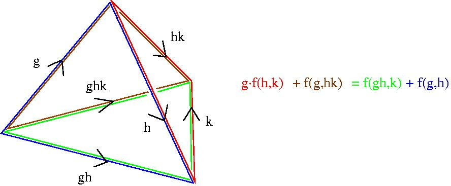
Given a ZG-resolution R_∗ and a ZG-module A, one defines an n-cocycle to be a ZG-homomorphism f: R_n → A for which the composite homomorphism fd_n+1: R_n+1→ A is zero. If R_∗ happens to be the standard bar resolution (i.e. the cellular chain complex of the nerve of the group G considered as a one object category) then the free ZG-generators of R_n are indexed by n-tuples (g_1 | g_2 | ... | g_n) of elements g_i in G. In this case we say that the n-cocycle is a standard n-cocycle and we think of it as a set-theoretic function
f : G × G × ⋯ × G ⟶ A
satisfying a certain algebraic cocycle condition. Bearing in mind that a standard n-cocycle really just assigns an element f(g_1, ... ,g_n) ∈ A to an n-simplex in the nerve of G , the cocycle condition is a very natural one which states that f must vanish on the boundary of a certain (n+1)-simplex. For n=2 the condition is that a 2-cocycle f(g_1,g_2) must satisfy
g.f(h,k) + f(g,hk) = f(gh,k) + f(g,h)
for all g,h,k ∈ G. This equation is explained by the following picture.
The definition of a cocycle clearly depends on the choice of ZG-resolution R_∗. However, the cohomology group H^n(G,A), which is a group of equivalence classes of n-cocycles, is independent of the choice of R_∗.
There are some occasions when one needs explicit examples of standard cocycles. For instance:
Let G be a finite group and k a field of characteristic 0. The group algebra k(G), and the algebra F(G) of functions d_g: G→ k, h→ d_g,h, are both Hopf algebras. The tensor product F(G) ⊗ k(G) also admits a Hopf algebra structure known as the quantum double D(G). A twisted quantum double D_f(G) was introduced by R. Dijkraaf, V. Pasquier & P. Roche [DPR91]. The twisted double is a quasi-Hopf algebra depending on a 3-cocycle f: G× G× G→ k. The multiplication is given by (d_g ⊗ x)(d_h ⊗ y) = d_gx,xhβ_g(x,y)(d_g ⊗ xy) where β_a is defined by β_a(h,g) = f(a,h,g) f(h,h^-1ah,g)^-1 f(h,g,(hg)^-1ahg) . Although the algebraic structure of D_f(G) depends very much on the particular 3-cocycle f, representation-theoretic properties of D_f(G) depend only on the cohomology class of f.
An explicit 2-cocycle f: G× G→ A is needed to construct the multiplication (a,g)(a',g') = (a + g⋅ a' + f(g,g'), gg') in the extension a group G by a ZG-module A determined by the cohomology class of f in H^2(G,A). See 6.7.
In work on coding theory and Hadamard matrices a number of papers have investigated square matrices (a_ij) whose entries a_ij=f(g_i,g_j) are the values of a 2-cocycle f: G× G → Z_2 where G is a finite group acting trivially on Z_2. See for instance [Hor00] and 6.10.
Given a ZG-resolution R_∗ (with contracting homotopy) and a ZG-module A one can use HAP commands to compute explicit standard n-cocycles f: G^n → A. With the twisted quantum double in mind, we illustrate the computation for n=3, G=S_3, and A=U(1) the group of complex numbers of modulus 1 with trivial G-action.
We first compute a ZG-resolution R_∗. The Universal Coefficient Theorem gives an isomorphism H_3(G,U(1)) = Hom_ Z(H_3(G, Z), U(1)), The multiplicative group U(1) can thus be viewed as Z_m where m is a multiple of the exponent of H_3(G, Z).
gap> G:=SymmetricGroup(3);;
gap> R:=ResolutionFiniteGroup(G,4);;
gap> TR:=TensorWithIntegers(R);;
gap> Homology(TR,3);
[ 6 ]
gap> R!.dimension(3);
4
gap> R!.dimension(4);
5
We thus replace the very infinite group U(1) by the finite cyclic group Z_6. Since the resolution R_∗ has 4 generators in degree 3, a homomorphism f: R^3→ U(1) can be represented by a list f=[f_1, f_2, f_3, f_4] with f_i the image in Z_6 of the ith generator. The cocycle condition on f can be expressed as a matrix equation
Mf^t = 0 mod 6.
where the matrix M is obtained from the following command and f^t denotes the transpose.
gap> M:=CocycleCondition(R,3);;
A particular cocycle f=[f_1, f_2, f_3, f_4] can be obtained by choosing a solution to the equation Mf^t=0.
gap> SolutionsMod2:=NullspaceModQ(TransposedMat(M),2);
[ [ 0, 0, 0, 0 ], [ 0, 0, 1, 1 ], [ 1, 1, 0, 0 ], [ 1, 1, 1, 1 ] ]

gap> SolutionsMod3:=NullspaceModQ(TransposedMat(M),3);
[ [ 0, 0, 0, 0 ], [ 0, 0, 0, 1 ], [ 0, 0, 0, 2 ], [ 0, 0, 1, 0 ],
  [ 0, 0, 1, 1 ], [ 0, 0, 1, 2 ], [ 0, 0, 2, 0 ], [ 0, 0, 2, 1 ],
  [ 0, 0, 2, 2 ] ]
A non-standard 3-cocycle f can be converted to a standard one using the command StandardCocycle(R,f,n,q) . This command inputs R_∗, integers n and q, and an n-cocycle f for the resolution R_∗. It returns a standard cocycle G^n → Z_q.
gap> f:=3*SolutionsMod2[3] - SolutionsMod3[5];   #An example solution to Mf=0 mod 6.
[ 3, 3, -1, -1 ]

gap> Standard_f:=StandardCocycle(R,f,3,6);;

gap> g:=Random(G); h:=Random(G); k:=Random(G);
(1,2)
(1,3,2)
(1,3)

gap> Standard_f(g,h,k);
3
A function f: G× G× G → A is a standard 3-cocycle if and only if
g⋅ f(h,k,l) - f(gh,k,l) + f(g,hk,l) - f(g,h,kl) + f(g,h,k) = 0
for all g,h,k,l ∈ G. In the above example the group G=S_3 acts trivially on A=Z_6. The following commands show that the standard 3-cocycle produced in the example really does satisfy this 3-cocycle condition.
gap> sf:=Standard_f;;

gap> Test:=function(g,h,k,l);
> return sf(h,k,l) - sf(g*h,k,l) + sf(g,h*k,l) - sf(g,h,k*l) + sf(g,h,k);
> end;
function( g, h, k, l ) ... end

gap> for g in G do for h in G do for k in G do for l in G do
> Print(Test(g,h,k,l),",");
> od;od;od;od;
0,0,0,0,0,0,0,0,0,0,0,0,0,0,0,0,0,0,0,0,0,0,0,0,0,0,0,0,0,0,0,0,0,0,0,0,0,0,
0,0,0,0,0,0,0,0,0,0,0,0,0,0,0,0,0,0,0,0,0,0,0,0,0,0,0,0,0,0,0,0,0,0,0,0,0,0,
0,0,0,0,0,0,0,0,0,0,0,0,0,0,0,0,0,0,0,0,0,0,0,0,0,0,0,0,0,0,0,0,0,0,0,0,0,0,
0,0,0,0,0,0,0,0,0,0,0,0,0,0,0,0,0,0,0,0,0,0,0,0,0,0,0,0,0,0,0,0,0,0,0,0,0,0,
0,0,0,0,0,0,0,0,0,0,0,0,0,0,0,0,0,0,0,0,0,0,0,0,0,0,0,0,0,0,0,0,0,0,0,0,0,0,
0,0,0,0,0,0,0,0,0,0,0,0,0,0,0,0,0,0,0,0,0,0,0,0,0,0,0,0,0,0,0,0,0,0,0,0,0,0,
0,0,0,0,0,0,0,0,0,0,0,0,0,0,0,0,0,0,0,0,0,0,0,0,0,0,0,0,0,0,0,6,0,6,6,0,0,6,
0,0,0,0,0,6,6,6,0,6,0,12,12,6,12,6,0,12,6,0,6,6,0,0,0,0,0,0,0,12,12,6,6,6,0,
6,6,0,6,6,0,0,-6,0,0,0,0,0,0,0,0,0,0,6,6,6,6,6,0,0,0,0,0,0,0,6,0,0,6,6,0,6,6,
0,6,0,0,6,6,6,0,0,0,0,0,0,0,-6,0,0,-6,0,-6,0,0,0,0,0,0,0,0,6,6,0,6,0,0,6,0,0,
0,0,0,6,6,6,0,0,0,6,6,6,0,0,0,0,-6,0,6,6,0,0,0,0,0,0,0,12,6,6,0,6,0,0,0,0,12,
6,0,0,0,0,0,0,0,6,6,0,0,0,0,0,0,0,0,0,0,0,0,0,0,0,0,0,0,0,0,0,0,0,0,0,0,0,0,
0,0,0,0,0,0,0,0,0,0,0,0,0,0,0,0,0,0,0,0,0,0,0,0,6,0,0,6,0,0,6,0,0,0,0,0,6,6,
6,0,0,0,6,12,6,6,0,0,0,-6,0,0,6,0,0,0,0,0,0,0,12,12,6,6,6,0,0,0,0,6,6,0,0,0,
0,0,0,0,0,0,0,0,0,0,0,0,0,0,0,0,0,0,0,0,0,0,0,0,0,0,6,0,0,6,0,6,0,0,0,0,0,0,
0,0,0,0,0,0,0,0,0,0,0,0,0,0,0,0,0,0,0,0,0,0,0,0,0,0,0,0,0,0,0,0,6,6,6,6,6,0,
6,6,0,6,6,0,12,12,6,12,12,0,0,0,0,0,0,0,6,6,0,0,0,0,6,6,6,12,12,0,-6,-6,0,0,
0,0,6,6,0,0,6,0,0,6,0,6,6,0,0,0,0,0,0,0,0,0,0,0,0,0,0,0,0,0,0,0,0,0,0,0,0,0,
0,0,0,0,0,0,0,0,0,0,0,0,0,0,0,0,0,0,6,0,6,0,0,0,0,0,0,0,0,0,0,0,0,0,0,0,6,6,
0,6,0,0,6,0,0,0,0,0,0,0,0,0,0,0,6,6,0,6,0,0,6,0,0,0,0,0,0,0,0,0,0,0,0,0,6,0,
0,0,0,0,0,0,0,0,0,0,0,0,0,0,6,0,0,6,6,0,6,6,0,6,0,0,6,6,6,0,0,0,0,0,0,0,0,0,
0,0,0,0,0,0,0,0,0,0,0,0,0,6,0,0,0,0,0,0,0,0,0,0,0,0,0,0,0,0,0,0,0,0,0,0,0,0,
0,6,6,0,0,0,0,0,0,0,0,0,0,0,0,0,0,0,0,6,6,0,0,0,0,0,0,0,6,6,0,0,0,0,0,0,0,0,
0,0,0,0,0,0,0,0,0,0,0,0,0,0,0,0,0,0,0,0,0,0,0,0,0,0,0,0,0,0,0,0,0,0,0,0,0,0,
0,0,0,0,0,0,0,0,0,0,-6,0,6,0,6,0,6,0,0,0,0,0,0,0,12,12,6,12,12,0,6,6,0,6,6,0,
0,0,0,0,0,0,12,12,6,12,12,0,6,6,0,6,6,0,0,0,0,0,0,0,0,0,0,0,0,0,6,6,6,6,6,0,
0,0,0,0,0,0,6,0,0,6,6,0,6,6,0,6,0,0,6,6,6,0,0,0,-6,0,0,0,-6,0,0,-6,0,-6,0,0,
0,0,0,0,0,0,0,0,0,0,0,0,0,0,0,0,0,0,6,6,6,6,6,0,6,6,0,0,0,0,0,0,0,6,6,0,0,0,
0,0,0,0,6,6,0,-6,0,0,-6,0,0,12,6,0,-6,-6,0,0,0,0,6,6,0,0,6,0,0,6,0,6,6,0,0,0,
0,0,0,0,0,0,0,0,0,0,0,0,0,0,0,0,0,0,0,0,0,0,0,0,0,0,0,0,0,0,0,0,0,0,0,0,0,0,
0,0,0,-6,0,0,0,0,0,0,0,0,0,0,6,6,6,6,6,0,6,12,0,6,0,0,6,0,0,0,6,0,0,0,0,0,0,
0,6,12,0,0,0,0,0,0,0,6,6,0,-6,-6,0,0,0,0,0,0,0,0,6,0,0,6,0,6,6,0,0,0,0,0,0,0,
6,0,0,0,6,0,0,6,0,6,0,0,0,0,0,0,0,0,0,0,0,0,0,0,0,0,0,0,0,0,0,0,0,0,0,0,0,6,
0,0,0,0,0,0,0,0,6,0,0,0,0,0,0,0,6,6,0,6,6,0,6,6,6,12,12,0,0,0,0,0,0,0,6,6,0,
6,6,0,6,6,6,12,12,0,0,0,0,0,0,0,6,6,0,0,6,0,0,6,0,6,6,
Let G be a finite group with order divisible by prime p. Let mathcal A=mathcal A_p(G) denote Quillen's simplicial complex arising as the order complex of the poset of non-trivial elementary abelian p-subgroups of G. The group G acts on mathcal A. Denote the orbit of a k-simplex e^k by [e^k], and the stabilizer of e^k by Stab(e^k) ≤ G. For a finite abelian group H let H_p denote the Sylow p-subgroup or the "p-part". In Theorem 3.3 of [Web87] P.J. Webb proved the following.
Theorem.[Web87] For any G-module M there is a (non natural) isomomorphism
H_n(G,M)_p ⊕ ⨁_[e^k] : k~ odd~H_n(Stab(e^k),M)_p ≅ ⨁_[e^k] : k~ even~H_n(Stab(e^k),M)_p
for n≥ 1. The isomorphism can also be expressed as
H_n(G,M)_p ≅ ⨁_[e^k] : k~ even~H_n(Stab(e^k),M)_p - ⨁_[e^k] : k~ odd~H_n(Stab(e^k),M)_p
where terms can often be cancelled.
Thus the additive structure of the p-part of the homology of G is determined by that of the stabilizer groups. The result also holds with homology replaced by cohomology.
Illustration 1
As an illustration of the theorem, the following commands calculate
H_n(SL_3( Z_2), Z) ≅ H_n(S_4, Z)_2 ⊕ H_n(S_4, Z)_2 ⊖ H_n(D_8, Z)_2 ⊕ H_n(S_3, Z)_3 ⊕ H_n(C_7 : C_3, Z)_7
where n≥ 1, S_k denotes the symmetric group on n letters, D_8 the dihedral group of order 8 and C_7 : C_3 a nonabelian semi-direct product of cyclic groups. Furthermore, for n≥ 1
H_n(C_7 : C_3, Z)_7 ={beginarrayll Z_7, n ≡ 5 mod 6 0, otherwise endarray.
and
H_n(S_3, Z)_3 ={beginarrayll Z_3, n ≡ 3 mod 4 0, n ~otherwise . endarray.
Formulas for H_n(S_4, Z) and H_n(D_8, Z) can be found in the literature. Alternatively, they can be computed using GAP for a given value of n. For n=27 we find
H_27(S_4, Z)_2 ⊕ H_27(S_4, Z)_2 ⊖ H_27(D_8, Z)_2 ≅ Z_2 ⊕ Z_2 ⊕ Z_2 ⊕ Z_2 ⊕ Z_4
and
H_27(SL_3( Z_2), Z) ≅ Z_2 ⊕ Z_2 ⊕ Z_2 ⊕ Z_2 ⊕ Z_4 ⊕ Z_3 .
gap> G:=SL(3,2);;Factors(Order(G));
[ 2, 2, 2, 3, 7 ]
gap> D2:=HomologicalGroupDecomposition(G,2);;
gap> D3:=HomologicalGroupDecomposition(G,3);;
gap> D7:=HomologicalGroupDecomposition(G,7);;
gap> List(D2[1],StructureDescription);
[ "S4", "S4" ]
gap> List(D2[2],StructureDescription);
[ "D8" ]
gap> List(D3[1],StructureDescription);
[ "S3" ]
gap> List(D3[2],StructureDescription);
[  ]
gap> List(D7[1],StructureDescription);
[ "C7 : C3" ]
gap> List(D7[2],StructureDescription);
[  ]

gap> CohomologicalPeriod(D7[1][1]);
6
gap> List([1..6],n->GroupHomology(D7[1][1],n));
[ [ 3 ], [  ], [ 3 ], [  ], [ 3, 7 ], [  ] ]

gap> CohomologicalPeriod(D3[1][1]);
4
gap> List([1..4],n->GroupHomology(D3[1][1],n));
[ [ 2 ], [  ], [ 6 ], [  ] ]

gap> R_S4:=ResolutionFiniteGroup(Group([(1,2),(2,3),(3,4)]),28);;
gap> R_D8:=ResolutionFiniteGroup(Group([(1,2),(1,3)(2,4)]),28);;

gap> Homology(TensorWithIntegers(R_S4),27);
[ 2, 2, 2, 2, 2, 2, 2, 2, 2, 12 ]
gap> Homology(TensorWithIntegers(R_D8),27);
[ 2, 2, 2, 2, 2, 2, 2, 2, 2, 2, 2, 2, 2, 2, 4 ]
Illustration 2
As a further illustration of the theorem, the following commands calculate
H_n(M_12,M)_3 ≅ ⨁_1≤ i≤ 3H_n(Stab_i,M)_3 - ⨁_4≤ i≤ 5H_n(Stab_i,M)_3
for the Mathieu simple group M_12 of order 95040, where
Stab_1≅ Stab_3=(((C_3 × C_3) : Q_8) : C_3) : C_2
Stab_2=A_4 × S_3
Stab_4=C_3 × S_3
Stab_5=((C_3 × C_3) : C_3) : (C_2 × C_2) .
gap> G:=MathieuGroup(12);;
gap> D:=HomologicalGroupDecomposition(G,3);;
gap> List(D[1],StructureDescription);
[ "(((C3 x C3) : Q8) : C3) : C2", "A4 x S3", "(((C3 x C3) : Q8) : C3) : C2" ]
gap> List(D[2],StructureDescription);
[ "C3 x S3", "((C3 x C3) : C3) : (C2 x C2)" ]
Illustration 3
As a third illustration, the following commands show that H_n(M_23,M)_p is periodic for primes p=5, 7, 11, 23 of periods dividing 8, 6, 10, 22 respectively. They also show that H_n(M_23, Z)_(3)=0 for n=8,9,12,13 and H_n(M_23, Z)_(3)= Z_3 for n=10,11.
gap> G:=MathieuGroup(23);;
gap> Factors(Order(G));
[ 2, 2, 2, 2, 2, 2, 2, 3, 3, 5, 7, 11, 23 ]

gap> sd:=StructureDescription;;

gap> D:=HomologicalGroupDecomposition(G,5);;
gap> List(D[1],sd);List(D[2],sd);
[ "C15 : C4" ]
[  ]
gap> IsPeriodic(D[1][1]);
true
gap> CohomologicalPeriod(D[1][1]);
8

gap> D:=HomologicalGroupDecomposition(G,7);;
gap> List(D[1],sd);List(D[2],sd);
[ "C2 x (C7 : C3)" ]
[  ]
gap> IsPeriodic(D[1][1]);
true
gap> CohomologicalPeriod(D[1][1]);
6

gap> D:=HomologicalGroupDecomposition(G,11);;
gap> List(D[1],sd);List(D[2],sd);
[ "C11 : C5" ]
[  ]
gap> IsPeriodic(D[1][1]);
true
gap> CohomologicalPeriod(D[1][1]);
10

gap> D:=HomologicalGroupDecomposition(G,23);;
gap> List(D[1],sd);List(D[2],sd);
[ "C23 : C11" ]
[  ]
gap> IsPeriodic(D[1][1]);
true
gap> CohomologicalPeriod(D[1][1]);
22
gap> G:=MathieuGroup(23);;
gap> D:=HomologicalGroupDecomposition(G,3);;
gap> List(D[1],StructureDescription);List(D[2],StructureDescription);
[ "(C3 x C3) : QD16", "A5 : S3" ]
[ "S3 x S3" ]
gap> for n in [8..13] do
> Print(List(D[1],g->GroupHomology(g,n))," , ",List(D[2],g->GroupHomology(g,n)),"\n\n");
> od;
[ [ 2, 2 ], [ 2, 2, 2 ] ] , [ [ 2, 2, 2, 2 ] ]

[ [ 2, 2, 2, 2 ], [ 2, 2, 2, 2 ] ] , [ [ 2, 2, 2, 2, 2, 2 ] ]

[ [ 2, 2, 3 ], [ 2, 2, 2, 3, 3 ] ] , [ [ 2, 2, 2, 2, 2, 3, 3 ] ]

[ [ 2, 2, 2, 8, 3 ], [ 2, 2, 2, 2, 4, 3, 3, 3, 3 ] ] ,
[ [ 2, 2, 2, 2, 2, 2, 2, 3, 3, 3, 3 ] ]

[ [ 2, 2, 2 ], [ 2, 2, 2, 2 ] ] , [ [ 2, 2, 2, 2, 2, 2 ] ]

[ [ 2, 2, 2, 2, 2 ], [ 2, 2, 2, 2, 2 ] ] , [ [ 2, 2, 2, 2, 2, 2, 2, 2 ] ]
The order |M_23|=10200960 is divisible by primes p=2, 3, 5, 7, 11, 23. For p=3 the following commands establish that the Poincare series
(x^16 - 2x^15 + 3x^14 - 4x^13 + 4x^12 - 4x^11 + 4x^10 - 3x^9 + 3x^8 - 3x^7 + 4x^6 - 4x^5 + 4x^4 -4x^3 + 3x^2 -2x + 1) / (x^18 - 2x^17 + 3x^16 - 4x^15 + 4x^14 - 4x^13 + 4x^12 - 4x^11 + 4x^10 - 4x^9 + 4x^8 - 4x^7 + 4x^6 - 4x^5 + 4x^4 - 4x^3 + 3x^2 - 2x + 1)
describes the dimension of the vector space H^n(M_23, Z_3) up to at least degree n=40. To prove that it describes the dimension in all degrees one would need to verify "completion criteria".
gap> G:=MathieuGroup(23);;
gap> D:=HomologicalGroupDecomposition(G,3);;
gap> List(D[1],StructureDescription);
[ "(C3 x C3) : QD16", "A5 : S3" ]
gap> List(D[2],StructureDescription);
[ "S3 x S3" ]

gap> P1:=PoincareSeriesPrimePart(D[1][1],3,40);
(x_1^16-2*x_1^15+3*x_1^14-4*x_1^13+4*x_1^12-4*x_1^11+4*x_1^10-3*x_1^9+3*x_1^8-3*x_1^7+4*x_1^6-4*x_1^5+\
4*x_1^4-4*x_1^3+3*x_1^2-2*x_1+1)/(x_1^18-2*x_1^17+3*x_1^16-4*x_1^15+4*x_1^14-4*x_1^13+4*x_1^12-4*x_1^1\
1+4*x_1^10-4*x_1^9+4*x_1^8-4*x_1^7+4*x_1^6-4*x_1^5+4*x_1^4-4*x_1^3+3*x_1^2-2*x_1+1)

gap> P2:=PoincareSeriesPrimePart(D[1][2],3,40);
(x_1^4-2*x_1^3+3*x_1^2-2*x_1+1)/(x_1^6-2*x_1^5+3*x_1^4-4*x_1^3+3*x_1^2-2*x_1+1)

gap> P3:=PoincareSeriesPrimePart(D[2][1],3,40);
(x_1^4-2*x_1^3+3*x_1^2-2*x_1+1)/(x_1^6-2*x_1^5+3*x_1^4-4*x_1^3+3*x_1^2-2*x_1+1)
Let A be the Lie algebra constructed from the associative algebra M^4× 4( Q) of all 4× 4 rational matrices. Let V be its adjoint module (with underlying vector space of dimension 16 and equal to that of A). The following commands compute H_4(A,V) = Q.
gap> M:=FullMatrixAlgebra(Rationals,4);;
gap> A:=LieAlgebra(M);;
gap> V:=AdjointModule(A);;
gap> C:=ChevalleyEilenbergComplex(V,17);;
gap> List([0..17],C!.dimension);
[ 16, 256, 1920, 8960, 29120, 69888, 128128, 183040, 205920, 183040, 128128,
  69888, 29120, 8960, 1920, 256, 16, 0 ]
gap> Homology(C,4);
1
Note that the eighth term C_8(V) in the Chevalley-Eilenberg complex C_∗(V) is a vector space of dimension 205920 and so it will take longer to compute the homology in degree 8.
As a second example, let B be the classical Lie ring of type B_3 over the ring of integers. The following commands compute H_3(B, Z)= Z ⊕ Z_2^105.
gap> A:=SimpleLieAlgebra("B",7,Integers);
<Lie algebra of dimension 105 over Integers>
gap> C:=ChevalleyEilenbergComplex(A,4,"sparse");
Sparse chain complex of length 4 in characteristic 0 .

gap> D:=ContractedComplex(C);
Sparse chain complex of length 4 in characteristic 0 .

gap> Collected(Homology(D,3));
[ [ 0, 1 ], [ 2, 105 ] ]
A short exact sequence of Lie algebras
M ↣ C ↠ L
(over a field k) is said to be a stem extension of L if M lies both in the centre Z(C) and in the derived subalgeba C^2. If, in addition, the rank of the vector space M is equal to the rank of the second Chevalley-Eilenberg homology H_2(L,k) then the Lie algebra C is said to be a cover of L.
Each finite dimensional Lie algebra L admits a cover C, and this cover can be shown to be unique up to Lie isomorphism.
The cover can be used to determine whether there exists a Lie algebra E whose central quotient E/Z(E) is isomorphic to L. The image in L of the centre of C is called the Lie Epicentre of L, and this image is trivial if and only if such an E exists.
The cover can also be used to determine the stem extensions of L. It can be shown that each stem extension is a quotient of the cover by an ideal in the Lie multiplier H_2(L,k).
The following commands compute the cover C of the solvable but non-nilpotent 13-dimensional Lie algebra L (over k= Q) that was introduced by M. Wuestner [Wue92]. They also show that: the second homology of C is trivial and compute the ranks of the homology groups in other dimensions; the Lie algebra L is not isomorphic to any central quotient E/Z(E).
gap> SCTL:=EmptySCTable(13,0,"antisymmetric");;
gap> SetEntrySCTable( SCTL, 1, 6, [ 1, 7 ] );;
gap> SetEntrySCTable( SCTL, 1, 8, [ 1, 9 ] );;
gap> SetEntrySCTable( SCTL, 1, 10, [ 1, 11 ] );;
gap> SetEntrySCTable( SCTL, 1, 12, [ 1, 13 ] );;
gap> SetEntrySCTable( SCTL, 1, 7, [ -1, 6 ] );;
gap> SetEntrySCTable( SCTL, 1, 9, [ -1, 8 ] );;
gap> SetEntrySCTable( SCTL, 1, 11, [ -1, 10 ] );;
gap> SetEntrySCTable( SCTL, 1, 13, [ -1, 12 ] );;
gap> SetEntrySCTable( SCTL, 6, 7, [ 1, 2 ] );;
gap> SetEntrySCTable( SCTL, 8, 9, [ 1, 3 ] );;
gap> SetEntrySCTable( SCTL, 6, 9, [ -1, 5 ] );;
gap> SetEntrySCTable( SCTL, 7, 8, [ 1, 5 ] );;
gap> SetEntrySCTable( SCTL, 2, 8, [ 1, 12 ] );;
gap> SetEntrySCTable( SCTL, 2, 9, [ 1, 13 ] );;
gap> SetEntrySCTable( SCTL, 3, 6, [ 1, 10 ] );;
gap> SetEntrySCTable( SCTL, 3, 7, [ 1, 11 ] );;
gap> SetEntrySCTable( SCTL, 2, 3, [ 1, 4 ] );;
gap> SetEntrySCTable( SCTL, 5, 6, [ -1, 12 ] );;
gap> SetEntrySCTable( SCTL, 5, 7, [ -1, 13 ] );;
gap> SetEntrySCTable( SCTL, 5, 8, [ -1, 10 ] );;
gap> SetEntrySCTable( SCTL, 5, 9, [ -1, 11 ] );;
gap> SetEntrySCTable( SCTL, 6, 11, [ -1/2, 4 ] );;
gap> SetEntrySCTable( SCTL, 7, 10, [ 1/2, 4 ] );;
gap> SetEntrySCTable( SCTL, 8, 13, [ 1/2, 4 ] );;
gap> SetEntrySCTable( SCTL, 9, 12, [ -1/2, 4 ] );;
gap> L:=LieAlgebraByStructureConstants(Rationals,SCTL);;

gap> C:=Source(LieCoveringHomomorphism(L));
<Lie algebra of dimension 15 over Rationals>

gap> Dimension(LieEpiCentre(L));
1

gap> ch:=ChevalleyEilenbergComplex(C,17);;
gap> List([0..16],n->Homology(ch,n));
[ 1, 1, 0, 9, 23, 27, 47, 88, 88, 47, 27, 23, 9, 0, 1, 1, 0 ]
generated by GAPDoc2HTML