|
1. Metrics on Vectors
|
The
data file contains a list L of
400 vectorsi in R3.
The following commands produce the 400×400 symmetric matrix whose
(i,j)-entry is the Manhattan distance between L[i] and L[j].
(Alternative choices of metric include the Euclidean squared metric and
Hamming metric.)
|
gap>
ReadPackage("hap","www/SideLinks/About/data.txt");
#This
reads
in
the
list
L
gap> S:=VectorsToSymmetricMatrix(L,ManhattanMetric);;
|
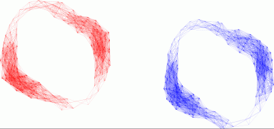
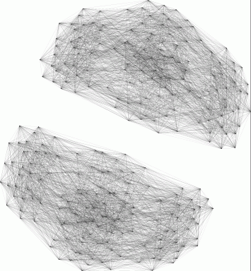
The
following command uses GraphViz software to display the graph G(S,t) on
400
vertices with edge between i and j precisely when
S[i][j] <= tM / 100
where M is the maximum value of the entries in S. Thus the threshold t
should be chosen in the range from 0 to 100. We choose t=8. We also
choose to give the first 200 vertices a common colour distinct from the
remaining vertices. The display shows that the first 200 vertices lie
in one path-component of G(S,8), and the remaining 200 vertices lie in
a second path-component. Each path-component "has the shape" of a
cylinder
or annulus.
|
gap>
SymmetricMatDisplay(S,8,
[
[1..200],
[201..400]
]
);
|
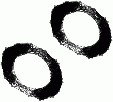
The
following commands construct the graph G=G(S,10) and then display it.
|
gap>
M:=Maximum(Maximum(S));;
gap> G:=SymmetricMatrixToGraph(S,10*M/100);
Graph on 400 vertices.
gap>
GraphDisplay(G);
|
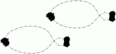
| We
use the term simplicial nerve
of G to mean the simplicial complex
NG which has the same vertices and edges as G; a collection of vertices
is a simplex in NG if and only if each pair of edges in the collection
is connected by an edge in G. The following commands determine a
subgraph H in G such that the simplicial nerves NG and NH are homotopy
equivalent. The commands replace G by H and then display the subgraph. |
gap>
ContractGraph(G);;
gap> G;
Graph on 248 vertices.
gap> GraphDisplay(G);
|
The
following commands illustrate two
methods for calculating the low-dimensional homology of NG. The second
method is more efficient in degrees 0 and 1 but has yet to be properly
implemented in higher degrees.
|
gap>
#Method
One
gap> NG:=SimplicialNerveOfGraph(G,3);;
gap> NG:=SimplicialComplexToRegularCWComplex(NG);
Regular CW-complex of dimension 3
gap> Homology(NG,0);
[ 0, 0 ]
gap> Homology(NG,1);
[ 0, 0 ]
gap> #Method Two
gap> C:=RipsChainComplex(G,1);
Sparse chain complex of length 2 in characteristic 0 .
gap> Bettinumbers(C,0);
2
gap> Bettinumbers(C,1);
2
|
2. Metrics on Permutations
|
There
are
a
number of standard metrics d(x,y) on permutations x, y such
as
the Kendall metric (=number of neighbouring
transpositions (i,i+1) needed to express x*y^-1), the Cayley metric (=
number of transpositions (i,j) needed to express x*y^-1) and the
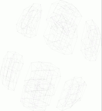
Hamming metric (= #{ i : x*y^-1(i) differs from i } ). The
following commands display the Sylow 2-subgroup of S10 with
respect to the Cayley metric.
|
gap>
G:=SymmetricGroup(10);;
gap> P:=SylowSubgroup(G,2);;
gap> P:=Elements(P);;
gap> S:=NullMat(Size(P),Size(P));;
gap> for i in [1..Size(P)] do
> for j in [1..Size(P)] do
> S[i][j]:=CayleyMetric(P[i],P[j],10);
> od;od;
gap> SymmetricMatDisplay(S,50);
gap> SymmetricMatDisplay(S,15);
|
|