| Previous |
About HAP: Digital Image Analysis |
next |
Pure cubical complex of dimension 3.
gap> Bettinumbers(M);
[ 1, 0, 0, 0 ]
Pure cubical complex of dimension 3.
gap> Bettinumbers(B);
[ 1, 0, 1, 0 ]
The function
SingularitiesOfPureCubicalComplex(M,radius,tolerance)
returns the space of singular points on the boundary of M. A boundary point is "singular" if the sphere of given radius around the point is divided into two equal sized components (up to some tolerance) by the boundary of M.
Pure cubical complex of dimension 3.
gap> Bettinumbers(S);
[ 1, 7, 0, 0 ]
In order to investigate the combinatorial type of the facets we form the pure cubical complex D=B-S of nonsingular boundary points of M, and determine the adjacency relation between the path components in the pure cubical complex D.
For example, the following commands show that there are eight path components in D (one for each facet), and that the first path component is adjacent to precisely four other path components.
gap> S:=SingularitiesOfPureCubicalComplex(M,3,15);;
gap> B:=BoundaryOfPureCubicalComplex(M);;
gap> D:=PureCubicalComplexDifference(B,S);
Pure cubical complex of dimension 3.
gap> Bettinumbers(D,0)); #Number of path componenets in D.
8
gap> P:=List([1..8],n->PathComponentOfPureCubicalComplex(D,n));;
gap> for n in [2..8] do
> U:=PureCubicalComplexUnion(P[1],P[n]);
> U:=ThickenedPureCubicalComplex(U);
> Print(Bettinumbers(U,1),"\n");
> od;
> U:=ThickenedPureCubicalComplex(P[1]);
> U:=ThickenedPureCubicalComplex(U);
> V:=ThickenedPureCubicalComplex(P[n]);
> V:=ThickenedPureCubicalComplex(V);
> W:=PureCubicalComplexIntersection(U,V);
> Print(Size(W),"\n");
> od;
128
95
95
50
0
0
0
A
2-dimensional
example
gap> for i in [1..15] do
> Print(Bettinumbers(T),"\n");
> T:=ThickenedPureCubicalComplex(T);;
> od;
[ 206, 5070, 0 ]
[ 11, 10, 0 ]
[ 4, 4, 0 ]
[ 3, 3, 0 ]
[ 3, 3, 0 ]
[ 3, 4, 0 ]
[ 3, 3, 0 ]
[ 3, 3, 0 ]
[ 3, 3, 0 ]
[ 3, 3, 0 ]
[ 3, 3, 0 ]
[ 3, 3, 0 ]
[ 3, 3, 0 ]
[ 3, 3, 0 ]
[ 3, 3, 0 ]
Space 1:
 Space 2:
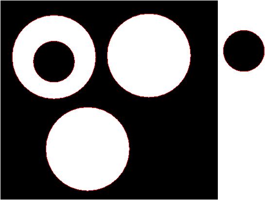
Space 3:
 Space
4:
Space
4:

Space 5:
By considering the betti numbers of the "inverted manifolds" obtained by inverting black and white, we can eliminate a few of these as possible ambient isotopy types for the digital photograph.
For example, the following commands show that the photograph is not ambient isotopic to manifolds 2, 3 or 5.
gap> for i in [1..8] do
> T:=ThickenedPureCubicalComplex(T);
> od;
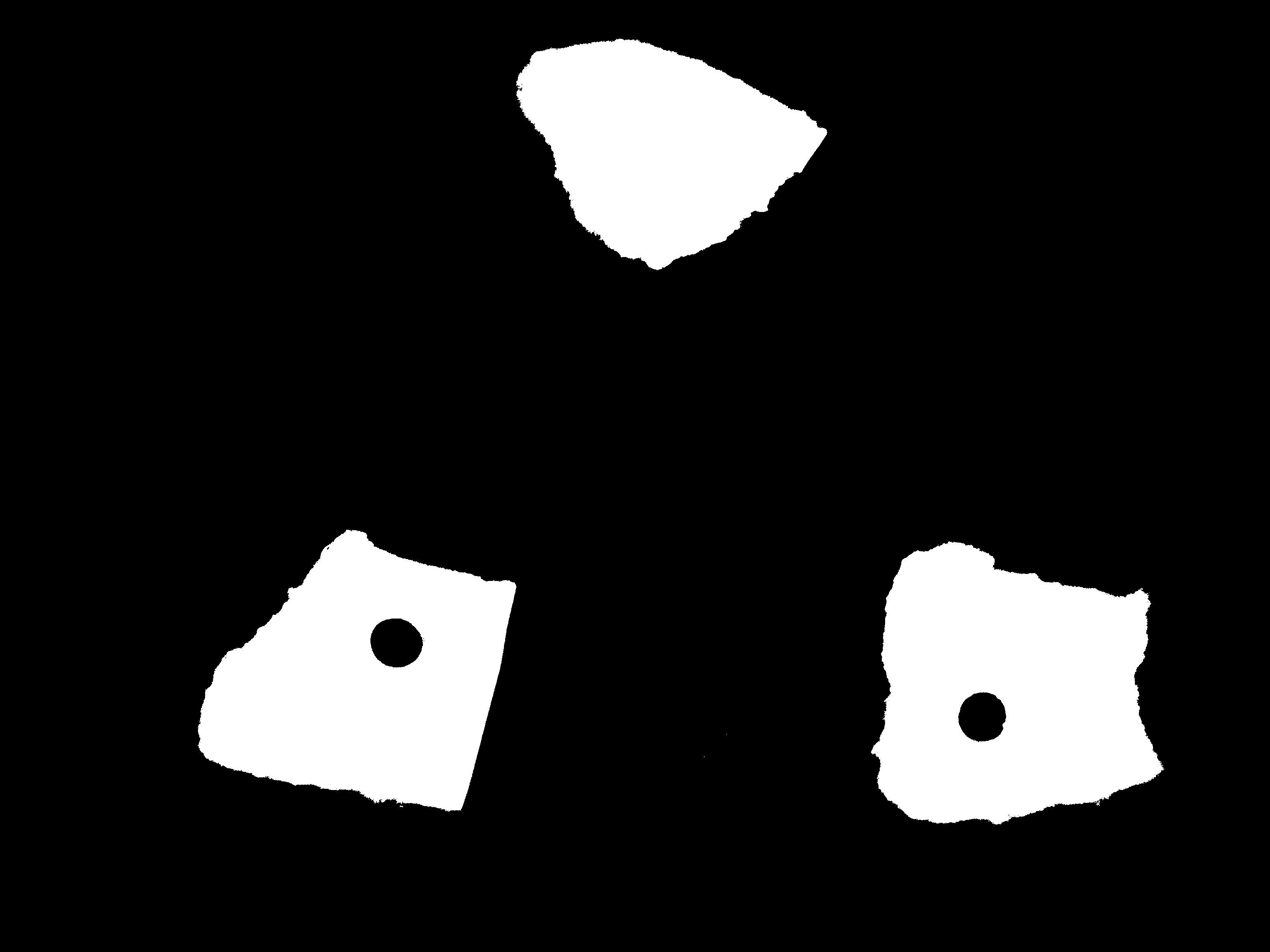
gap> T1:=ReadImageAsPureCubicalComplex("space1.jpg",400);;
gap> T2:=ReadImageAsPureCubicalComplex("space2.jpg",400);;
gap> T3:=ReadImageAsPureCubicalComplex("space3.jpg",400);;
gap> T4:=ReadImageAsPureCubicalComplex("space4.jpg",400);;
gap> T5:=ReadImageAsPureCubicalComplex("space5.jpg",400);;
gap> Bettinumbers(ComplementOfPureCubicalComplex(T));
[ 3, 2, 0 ]
gap> Bettinumbers(ComplementOfPureCubicalComplex(T1));
[ 3, 2, 0 ]
gap> Bettinumbers(ComplementOfPureCubicalComplex(T2));
[ 4, 3, 0 ]
gap> Bettinumbers(ComplementOfPureCubicalComplex(T3));
[ 4, 2, 0 ]
gap> Bettinumbers(ComplementOfPureCubicalComplex(T4));
[ 3, 2, 0 ]
gap> Bettinumbers(ComplementOfPureCubicalComplex(T5));
[ 4, 3, 0 ]
gap> Bettinumbers(T1)[1];
3
gap> Bettinumbers(PathComponentOfPureCubicalComplex(T1,1));
[ 1, 3, 0 ]
gap> Bettinumbers(PathComponentOfPureCubicalComplex(T1,2));
[ 1, 0, 0 ]
gap> Bettinumbers(PathComponentOfPureCubicalComplex(T1,3));
[ 1, 0, 0 ]
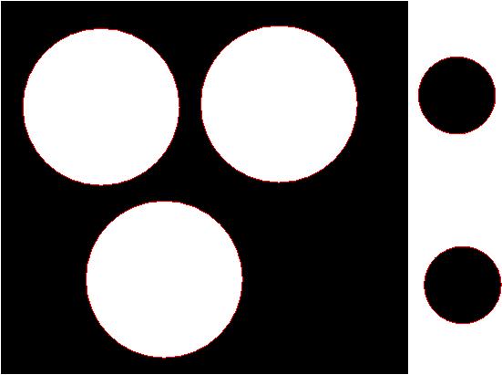
gap> T4:=ReadImageAsPureCubicalComplex("space4.jpg",400);;
gap> Bettinumbers(PathComponentOfPureCubicalComplex(T4,1));
[ 1, 2, 0 ]
gap> Bettinumbers(PathComponentOfPureCubicalComplex(T4,2));
[ 1, 1, 0 ]
gap> Bettinumbers(PathComponentOfPureCubicalComplex(T4,3));
[ 1, 0, 0 ]
| Previous
Page |
Contents |
Next
page |