The following example uses the nonabelian tensor square of groups to compute the third homotopy group
\(\pi_3(S(K(G,1))) = \mathbb Z^{30}\)
of the suspension of the Eigenberg-MacLane space \(K(G,1)\) for \(G\) the free nilpotent group of class \(2\) on four generators.
gap> F:=FreeGroup(4);;G:=NilpotentQuotient(F,2);;
gap> ThirdHomotopyGroupOfSuspensionB(G);
[ 0, 0, 0, 0, 0, 0, 0, 0, 0, 0, 0, 0, 0, 0, 0, 0, 0, 0, 0, 0, 0, 0,
  0, 0, 0, 0, 0, 0, 0, 0 ]
The following example constructs the finitely presented quandles associated to the granny knot and square knot, and then computes the number of quandle homomorphisms from these two finitely prresented quandles to the \(17\)-th quandle in HAP's library of connected quandles of order \(24\). The number of homomorphisms differs between the two cases. The computation therefore establishes that the complement in \(\mathbb R^3\) of the granny knot is not homeomorphic to the complement of the square knot.
gap> Q:=ConnectedQuandle(24,17,"import");;
gap> K:=PureCubicalKnot(3,1);;
gap> L:=ReflectedCubicalKnot(K);;
gap> square:=KnotSum(K,L);;
gap> granny:=KnotSum(K,K);;
gap> gcsquare:=GaussCodeOfPureCubicalKnot(square);;
gap> gcgranny:=GaussCodeOfPureCubicalKnot(granny);;
gap> Qsquare:=PresentationKnotQuandle(gcsquare);;
gap> Qgranny:=PresentationKnotQuandle(gcgranny);;
gap> NumberOfHomomorphisms(Qsquare,Q);
408
gap> NumberOfHomomorphisms(Qgranny,Q);
24
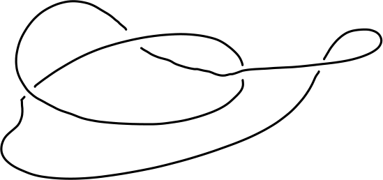
The following commands compute a knot quandle directly from a pdf file containing the following hand-drawn image of the knot.
gap>  gc:=ReadLinkImageAsGaussCode("myknot.pdf");
[ [ [ -2, 4, -1, 3, -3, 2, -4, 1 ] ], [ -1, -1, 1, -1 ] ]
gap> Q:=PresentationKnotQuandle(gc);
Quandle presentation of 4 generators and 4 relators.
Low index subgrops of the knot group can be used to identify knots with few crossings. For instance, the following commands read in the following image of a knot and identify it as a sum of two trefoils. The commands determine the prime components only up to reflection, and so they don't distinguish between the granny and square knots.
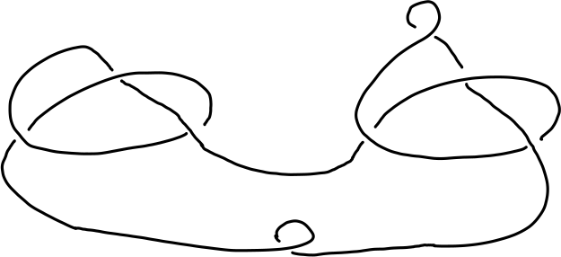
gap> gc:=ReadLinkImageAsGaussCode("myknot2.png");
[ [ [ -4, 7, -5, 4, -7, 5, -3, 6, -2, 3, 8, -8, -6, 2, 1, -1 ] ],
  [ 1, -1, -1, -1, -1, -1, -1, 1 ] ]
gap> IdentifyKnot(gc);;
PrimeKnot(3,1) + PrimeKnot(3,1)    modulo reflections of components.
The following example uses Polymake's linear programming routines to establish that the \(2\)-complex associated to the group presentation \(<x,y,z : xyx=yxy,\, yzy=zyz,\, xzx=zxz>\) is aspherical (that is, has contractible universal cover). The presentation is Tietze equivalent to the presentation used in the computer code, and the associated \(2\)-complexes are thus homotopy equivalent.
gap> F:=FreeGroup(6);;
gap> x:=F.1;;y:=F.2;;z:=F.3;;a:=F.4;;b:=F.5;;c:=F.6;;
gap> rels:=[a^-1*x*y, b^-1*y*z, c^-1*z*x, a*x*(y*a)^-1,
>    b*y*(z*b)^-1, c*z*(x*c)^-1];;
gap> Print(IsAspherical(F,rels),"\n");
Presentation is aspherical.

true
Free resolutons for a group \(G\) are constructed in HAP as the cellular chain complex \(R_\ast=C_\ast(\tilde X)\) of the universal cover of some CW-complex \(X=K(G,1)\). The \(2\)-skeleton of \(X\) gives rise to a free presentation for the group \(G\). This presentation depends on a choice of maximal tree in the \(1\)-skeleton of \(X\) in cases where \(X\) has more than one \(0\)-cell. The attaching maps of \(3\)-cells in \(X\) can be regarded as homotopical syzygies or van Kampen diagrams over the group presentation whose boundaries spell the trivial word.
The following example constructs four terms of a resolution for the free abelian group \(G\) on \(n=3\) generators, and then extracts the group presentation from the resolution as well as the unique homotopical syzygy. The syzygy is visualized in terms of its graph of edges, directed edges being coloured according to the corresponding group generator. (In this example the CW-complex \(\tilde X\) is regular, but in cases where it is not the visualization may be a quotient of the \(1\)-skeleton of the syzygy.)
gap> n:=3;;c:=1;;
gap> G:=Image(NqEpimorphismNilpotentQuotient(FreeGroup(n),c));;
gap> R:=ResolutionNilpotentGroup(G,4);;
gap> P:=PresentationOfResolution(R);;
gap> P.freeGroup;
<free group on the generators [ x, y, z ]>
gap> P.relators;
[ y^-1*x^-1*y*x, z^-1*x^-1*z*x, z^-1*y^-1*z*y ]
gap> IdentityAmongRelatorsDisplay(R,1);
This homotopical syzygy represents a relationship between the three relators \([x,y]\), \([x,z]\) and \([y,z]\) where \([x,y]=xyx^{-1}y^{-1}\). The syzygy can be thought of as a geometric relationship between commutators corresponding to the well-known Hall-Witt identity:
\( [\ [x,y],\ {^yz}\ ]\ \ [\ [y,z],\ {^zx}\ ]\ \ [\ [z,x],\ {^xy}\ ]\ \ =\ \ 1\ \ .\)
The homotopical syzygy is special since in this example the edge directions and labels can be understood as specifying three homeomorphisms between pairs of faces. Viewing the syzygy as the boundary of the \(3\)-ball, by using the homeomorphisms to identify the faces in each face pair we obtain a quotient CW-complex \(M\) involving one vertex, three edges, three \(2\)-cells and one \(3\)-cell. The cell structure on the quotient exists because, under the restrictions of homomorphisms to the edges, any cycle of edges retricts to the identity map on any given edge. The following result tells us that \(M\) is in fact a closed oriented compact \(3\)-manifold.
Theorem. [Seifert u. Threlfall, Topologie, p.208] Let \(S^2\) denote the boundary of the \(3\)-ball \(B^3\) and suppose that the sphere \(S^2\) is given a regular CW-structure in which the faces are partitioned into a collection of face pairs. Suppose that for each face pair there is an orientation reversing homeomorphism between the two faces that sends edges to edges and vertices to vertices. Suppose that by using these homeomorphisms to identity face pairs we obtain a (not necessarily regular) CW-structure on the quotient \(M\). Then \(M\) is a closed compact orientable manifold if and only if its Euler characteristic is \(\chi(M)=0\).
The next commands construct a presentation and associated unique homotopical syzygy for the free nilpotent group of class \(c=2\) on \(n=2\) generators.
gap> n:=2;;c:=2;;
gap> G:=Image(NqEpimorphismNilpotentQuotient(FreeGroup(n),c));;
gap> R:=ResolutionNilpotentGroup(G,4);;
gap> P:=PresentationOfResolution(R);;
gap> P.freeGroup;
<free group on the generators [ x, y, z ]>
gap> P.relators;
[ z*x*y*x^-1*y^-1, z*x*z^-1*x^-1, z*y*z^-1*y^-1 ]
gap> IdentityAmongRelatorsDisplay(R,1);
The syzygy represents the following relationship between commutators (in a free group).
\( [\ [x^{-1},y][x,y]\ ,\ [y,x][y^{-1},x]y^{-1}\ ]\ [\ [y,x][y^{-1},x]\ , \ x^{-1} \ ] \ \ =\ \ 1\)
Again, using the theorem of Seifert and Threlfall we see that the free nilpotent group of class two on two generators arises as the fundamental group of a closed compact orientable \(3\)-manifold \(M\).
The Bogomolov multiplier of a group is an isoclinism invariant. Using this property, the following example shows that there are precisely three groups of order \(243\) with non-trivial Bogomolov multiplier. The groups in question are numbered 28, 29 and 30 in GAP's library of small groups of order \(243\).
gap> L:=AllSmallGroups(3^5);;
gap> C:=IsoclinismClasses(L);;
gap> for c in C do
> if Length(BogomolovMultiplier(c[1]))>0 then
> Print(List(c,g->IdGroup(g)),"\n\n\n"); fi;
> od;
[ [ 243, 28 ], [ 243, 29 ], [ 243, 30 ] ]
Any group extension \(N\rightarrowtail E \twoheadrightarrow G\) gives rise to:
an outer action \(\alpha\colon G\rightarrow Out(N)\) of \(G\) on \(N\).
an action \(G\rightarrow Aut(Z(N))\) of \(G\) on the centre of \(N\), uniquely induced by the outer action \(\alpha\) and the canonical action of \(Out(N)\) on \(Z(N)\).
a "\(2\)-cocycle" \(f\colon G\times G\rightarrow N\).
Any outer homomorphism \(\alpha\colon G\rightarrow Out(N)\) gives rise to a cohomology class \(k\) in \(H^3(G,Z(N))\). It was shown by Eilenberg and Mac\(\,\)Lane that the class \(k\) is trivial if and only if the outer action \(\alpha\) arises from some group extension \(N\rightarrowtail E\twoheadrightarrow G\). If \(k\) is trivial then there is a (non-canonical) bijection between the second cohomology group \(H^2(G,Z(N))\) and Yoneda equivalence classes of extensions of \(G\) by \(N\) that are compatible with \(\alpha\).
First Example.
Consider the group \(H=SmallGroup(64,134)\). Consider the normal subgroup \(N=NormalSubgroups(G)[15]\) and quotient group \(G=H/N\). We have \(N=C_2\times D_4\), \(A=Z(N)=C_2\times C_2\) and \(G=C_2\times C_2\).
Suppose we wish to classify all extensions \(C_2\times D_4 \rightarrowtail E \twoheadrightarrow C_2\times C_2\) that induce the given outer action of \(G\) on \(N\). The following commands show that, up to Yoneda equivalence, there are two such extensions.
gap> H:=SmallGroup(64,134);;
gap> N:=NormalSubgroups(H)[15];;
gap> A:=Centre(GOuterGroup(H,N));;
gap> G:=ActingGroup(A);;
gap> R:=ResolutionFiniteGroup(G,3);;
gap> C:=HomToGModule(R,A);;
gap> Cohomology(C,2);
[ 2 ]
The following additional commands return a standard \(2\)-cocycle \(f:G\times G\rightarrow A =C_2\times C_2\) corresponding to the non-trivial element in \(H^2(G,A)\). The value \(f(g,h)\) of the \(2\)-cocycle is calculated for all \(16\) pairs \(g,h \in G\).
gap> CH:=CohomologyModule(C,2);;
gap> Elts:=Elements(ActedGroup(CH));
[ <identity> of ..., f1 ]

gap> x:=Elts[2];;
gap> c:=CH!.representativeCocycle(x);
Standard 2-cocycle

gap> f:=Mapping(c);;
gap> for g in G do for h in G do
> Print(f(g,h),"\n");
> od;
> od;
<identity> of ...
<identity> of ...
<identity> of ...
<identity> of ...
<identity> of ...
f6
<identity> of ...
f6
<identity> of ...
<identity> of ...
<identity> of ...
<identity> of ...
<identity> of ...
f6
<identity> of ...
f6
The following commands will then construct and identify all extensions of \(N\) by \(G\) corresponding to the given outer action of \(G\) on \(N\).
gap> H := SmallGroup(64,134);;
gap> N := NormalSubgroups(H)[15];;
gap> ON := GOuterGroup(H,N);;
gap> A := Centre(ON);;
gap> G:=ActingGroup(A);;
gap> R:=ResolutionFiniteGroup(G,3);;
gap> C:=HomToGModule(R,A);;
gap> CH:=CohomologyModule(C,2);;
gap> Elts:=Elements(ActedGroup(CH));;

gap> lst := List(Elts{[1..Length(Elts)]},x->CH!.representativeCocycle(x));;
gap> ccgrps := List(lst, x->CcGroup(ON, x));;
gap> #So ccgrps is a list of groups, each being an extension of G by N, corresponding
gap> #to the two elements in H^2(G,A).

gap> #The following command produces the GAP identification number for each group.
gap> L:=List(ccgrps,IdGroup);
[ [ 64, 134 ], [ 64, 135 ] ]
Second Example
The following example illustrates how to construct a cohomology class \(k\) in \(H^2(G, A)\) from a cocycle \(f:G \times G \rightarrow A\), where \(G=SL_2(\mathbb Z_4)\) and \(A=\mathbb Z_8\) with trivial action.
gap> #We'll construct G=SL(2,Z_4) as a permutation group.
gap> G:=SL(2,ZmodnZ(4));;
gap> G:=Image(IsomorphismPermGroup(G));;

gap> #We'll construct Z_8=Z/8Z as a G-outer group
gap> z_8:=Group((1,2,3,4,5,6,7,8));;
gap> Z_8:=TrivialGModuleAsGOuterGroup(G,z_8);;

gap> #We'll compute the group h=H^2(G,Z_8)
gap> R:=ResolutionFiniteGroup(G,3);;  #R is a free resolution
gap> C:=HomToGModule(R,Z_8);; # C is a chain complex
gap> H:=CohomologyModule(C,2);; #H is the second cohomology H^2(G,Z_8)
gap> h:=ActedGroup(H);; #h is the underlying group of H

gap> #We'll compute  cocycles c2, c5 for the second and fifth cohomology classs
gap> c2:=H!.representativeCocycle(Elements(h)[2]);
Standard 2-cocycle

gap> c5:=H!.representativeCocycle(Elements(h)[5]);
Standard 2-cocycle

gap> #Now we'll construct the cohomology classes C2, C5 in the group h corresponding to the cocycles c2, c5.
gap> C2:=CohomologyClass(H,c2);;
gap> C5:=CohomologyClass(H,c5);;

gap> #Finally, we'll show that C2, C5 are distinct cohomology classes, both of order 4.
gap> C2=C5;
false
gap> Order(C2);
4
gap> Order(C5);
4
GAP offers a number of data types for representing groups, including those of fp-groups (finitely presented groups), pc-groups (power-conjugate presentated groups for finite polycyclic groups), pcp-groups (polycyclically presented groups for finite and infinite polycyclic groups), permutation groups (for finite groups), and matrix groups over a field or ring. Each data type has its advantages and limitations.
Based on the definitions and examples in Section 6.7 the additional data type of a cc-group (cocyclic group) is provided in HAP. This can be used for a group \(E\) arising as a group extension \(N\rightarrowtail E \twoheadrightarrow G\) and is a component object involving:
E!.Base consisting of some representation of a group \(G\).
E!.Fibre consisting of some representation of a group \(N\).
E!.OuterGroup consisting of an outer action \(\alpha\colon G\rightarrow Out(N)\) of \(G\) on \(N\).
E!.Cocycle consisting of a "\(2\)-cocycle" \(f\colon G\times G\rightarrow N\).
The first example in Section 6.7 illustrates the construction of cc-groups for which both the base \(G\) and fibre \(N\) are finite pc-groups. That example extends to any scenario in which the base \(G\) is a group for which:
we can construct the first 3 degrees of a free \(\mathbb ZG\)-resolution \(C_\ast X\).
we can construct the first 2 terms of a contracting homotopy \(h_i\colon C_nX\rightarrow C_{n+1}X \) for \(i=0,1\).
\(N\) is a group in which we can multiply elements effectively and for which we can determine the centre \(Z(N)\) and outer automorphism group \(Out(N)\).
As an illustration where the base group is a non-solvable finite group and the fibre is the infinite cyclic group, with base group acting trivially on the fibre, the following commands list up to Yoneda equivalence all central extensions \(\mathbb Z \rightarrowtail E \twoheadrightarrow G\) for \(G=A_5:C_{16}\). The base group is a non-solvable semi-direct product of order \(960\) and thus none of the \(16\) extensions are polycyclic. The commands classify the extensions according to their integral homology in degrees \( \le 2\), showing that there are precisely 5 such equivalence classes of extensions. Thus, there are at least 5 distinct isomorphism types among the \(16\) extensions. A presentation is constructed for the group corresponding to the sixteenth extension. The final command lists the orders of the 16 cohomology group elements corresponding to the 16 extensions. The 16th element has order 1, meaning that the sixteenth extension is the direct product \(C_\infty\ \times\ A_5:C_{16}\).
gap> G:=SmallGroup(960,637);;
gap> StructureDescription(G);
"A5 : C16"

gap> N:=AbelianPcpGroup([0]);;
gap> N:=TrivialGModuleAsGOuterGroup(G,N);;
gap> R:=ResolutionFiniteGroup(G,3);;
gap> C:=HomToGModule(R,N);;
gap> CH:=CohomologyModule(C,2);;
gap> Elts:=Elements(ActedGroup(CH));;
gap> lst := List(Elts{[1..Length(Elts)]},x->CH!.representativeCocycle(x));;
gap> ccgrps := List(lst, x->CcGroup(N, x));;

gap> inv:=function(gg)
> local T;
> T:=ResolutionInfiniteCcGroup(gg,3);
> return List([1..2],i->Homology(TensorWithIntegers(T),i));
> end;;

gap> EquivClasses:=Classify(ccgrps,inv);
 [ <Cc-group of Size infinity>, <Cc-group of Size infinity>,
      <Cc-group of Size infinity>, <Cc-group of Size infinity>,
      <Cc-group of Size infinity>, <Cc-group of Size infinity>,
      <Cc-group of Size infinity>, <Cc-group of Size infinity> ],
  [ <Cc-group of Size infinity>, <Cc-group of Size infinity>,
      <Cc-group of Size infinity>, <Cc-group of Size infinity> ],
  [ <Cc-group of Size infinity>, <Cc-group of Size infinity> ],
  [ <Cc-group of Size infinity> ], [ <Cc-group of Size infinity> ] ]
gap> List(EquivClasses,Size);
[ 8, 4, 2, 1, 1 ]

gap> F16:=Image(IsomorphismFpGroup(ccgrps[16]));
<fp group on the generators [ x, y, z, w, v ]>
gap> RelatorsOfFpGroup(F16);
[ (x^2*y*z*w*z*y)^3*x^2*(y*x*w*y^2*z*x*y*z*y)^3*y*x*w*y^2*z*x*y^2*z*w*y^2*z*y,
  x*y^-2*w^-1*z^-1*y^-1*x^-1*y, x*z^-1*y^-1*z^-1*w^-1*z^-1*y^-1*x^-1*z,
  x*y^-2*z^-1*w^-1*z^-1*y^-1*x^-1*w, z^-2, w^-2, y^-3, w*y^-1*w^-1*y^-1,
  w*z*w^-1*z^-1*w^-1*z, z*y^2*(z^-1*y^-1)^2, v^-1*x^-1*v*x, v*y*v^-1*y^-1,
  v*z*v^-1*z^-1, v*w*v^-1*w^-1 ]

gap> List(Elts,Order);
[ 16, 16, 16, 16, 16, 16, 16, 16, 8, 8, 8, 8, 4, 4, 2, 1 ]
For any free \(\mathbb ZG\)-resolution \(R_\ast=C_\ast X\) arising as the cellular chain complex of a contractible CW-complex, the terms in degrees \(\le 2\) correspond to a free presentation for the group \(G\). The following example accesses this presentation for the group \(PGL_3(\mathbb Z[\sqrt{-1}])\).
gap> K:=ContractibleGcomplex("PGL(3,Z[i])");;
gap> R:=FreeGResolution(K,2);;
gap> P:=PresentationOfResolution(R);;
gap> G:=P.freeGroup/P.relators;
<fp group on the generators [ v, w, x, y, z ]>
gap> P.relators;
[ v^2, w^-1*v*w*v^-1, w^-1*v^-1*w^-1, (x^-1*w)^3, (y^-1*w)^3, (z^-1*w)^4,
  y^-1*v^-1*z*y^-1*x, y^-1*v*x*v^-1*x*v, v^-1*z*v^-1*x*y, v^-1*x*v*y*v*x*v*y,
  x^3, x*z*y, y^-1*v^-1*y^2*v*y^-1, (v*y)^4, z^-1*y*v*z^-1, (v*y*z)^2,
  v^-1*(z*v)^2*z ]
The homomorphism \(h_0\colon R_0 \rightarrow R_1\) of a contracting homotopy provides a unique expression for each element of \(G\) as a word in the free generators. To illustrate this, we consider the Sylow \(2\)-subgroup \(H=Syl_2(M_{24})\) of the Mathieu group \(M_{24}\). We obtain a resolution \(R_\ast\) for \(H\) by recursively applying perturbation techniques to a composition series for \(H\). Such a resolution will yield a "kind of" power-conjugate presentation for \(H\).
gap> H:=SylowSubgroup(MathieuGroup(24),2);
<permutation group of size 1024 with 10 generators>
gap> Order(H);
1024
gap> C:=CompositionSeries(H);;
gap> R:=ResolutionSubnormalSeries(C,2);;
gap> P:=PresentationOfResolution(R);;
gap> P.freeGroup/P.relators;
<fp group on the generators [ q, r, s, t, u, v, w, x, y, z ]>
gap> P.relators;
[ q^-2*z*y*x*w*v, q*r^-1*q^-1*y*u*r, s*q*s^-1*q^-1, t*q*t^-1*q^-1,
  q*u^-1*q^-1*y*v*u, y*q*v^-1*q^-1, q*w^-1*q^-1*z*x, w*q*x^-1*q^-1,
  q*y^-1*q^-1*z*v, z*q*z^-1*q^-1, r^-2, t*r*s^-1*r^-1, s*r*t^-1*r^-1,
  u*r*u^-1*r^-1, v*r*v^-1*r^-1, r*w^-1*r^-1*y*w*u, r*x^-1*r^-1*y*x*u,
  y*r*y^-1*r^-1, z*r*z^-1*r^-1, s^-2, t*s*t^-1*s^-1, x*s*u^-1*s^-1,
  s*v^-1*s^-1*z*y*w*u, s*w^-1*s^-1*y*v*u, u*s*x^-1*s^-1, s*y^-1*s^-1*y*x*u,
  z*s*z^-1*s^-1, t^-2, t*u^-1*t^-1*y*x*u, t*v^-1*t^-1*z*w, t*w^-1*t^-1*z*v,
  y*t*x^-1*t^-1, x*t*y^-1*t^-1, z*t*z^-1*t^-1, u^-2, v*u*v^-1*u^-1,
  u*w^-1*u^-1*z*w, x*u*x^-1*u^-1, y*u*y^-1*u^-1, z*u*z^-1*u^-1, v^-2,
  w*v*w^-1*v^-1, v*x^-1*v^-1*z*x, y*v*y^-1*v^-1, z*v*z^-1*v^-1, w^-2,
  x*w*x^-1*w^-1, w*y^-1*w^-1*z*y, z*w*z^-1*w^-1, x^-2, y*x*y^-1*x^-1,
  z*x*z^-1*x^-1, y^-2, z*y*z^-1*y^-1, z^-2 ]
The following additional commands use the contracting homotopy homomorphism \(h_0\colon R_0\rightarrow R_1\) to express some random elements of \(H\) as words in the free generators.
gap> g:=Random(H);
(1,6)(2,3)(4,9)(5,16)(7,10)(8,21)(11,18)(12,17)(13,19)(14,20)(15,22)(23,24)
gap> P.wordInFreeGenerators(g);
q^-1*t^-1*x^-1*y^-1
gap>
gap> g:=Random(H);
(1,6)(2,23,10,18)(3,22,19,24)(4,11,15,9)(7,8,21,13)(12,14)
gap> P.wordInFreeGenerators(g);
q^-1*u^-1*w^-1*x^-1*z^-1
gap>
gap> g:=Random(H);
(1,14,5,17)(2,7,9,19)(3,11,4,22)(6,12,16,20)(8,18,24,15)(10,23,13,21)
gap> P.wordInFreeGenerators(g);
q^-1*r^-1*t^-1*v^-1*x^-1*z^-1
gap>
gap> g:=Random(H);
(1,14,5,17)(2,21)(3,9)(4,24)(6,12,16,20)(7,11,15,13)(8,23)(10,18,22,19)
gap> P.wordInFreeGenerators(g);
q^-1*r^-1*t^-1*v^-1*w^-1*z^-1
Because the resolution \(R_\ast\) was obtained from a composition series, the unique word associated to an element \(g\in H\) always has the form \(q^{\epsilon_1} r^{\epsilon_2} s^{\epsilon_3} t^{\epsilon_4} u^{\epsilon_5} v^{\epsilon_6} w^{\epsilon_7} x^{\epsilon_8} y^{\epsilon_9} z^{\epsilon_{10}}\) determined by the exponent vector \((\epsilon_1,\cdots,\epsilon_{10}) \in (\mathbb Z_2)^{10}\).
An Hadamard matrix is a square \(n\times n\) matrix \(H\) whose entries are either \(+1\) or \(-1\) and whose rows are mutually orthogonal, that is \(H H^t = nI_n\) where \(H^t\) denotes the transpose and \(I_n\) denotes the \(n\times n\) identity matrix.
Given a group \(G=\{g_1,g_2,\ldots,g_n\}\) of order \(n\) and the abelian group \(A=\{1,-1\}\) of square roots of unity, any \(2\)-cocycle \(f\colon G\times G\rightarrow A\) corresponds to an \(n\times n\) matrix \(F=(f(g_i,g_j))_{1\le i,j\le n}\) whose entries are \(\pm 1\). If \(F\) is Hadamard it is called a cocyclic Hadamard matrix corresponding to \(G\).
The following commands compute all \(192\) of the cocyclic Hadamard matrices for the abelian group \(G=\mathbb Z_4\oplus \mathbb Z_4\) of order \(n=16\).
gap> G:=AbelianGroup([4,4]);;
gap> F:=CocyclicHadamardMatrices(G);;
gap> Length(F);
192
Homotopy 2-types
The third cohomology \(H^3(G,A)\) of a group \(G\) with coefficients in a \(G\)-module \(A\), together with the corresponding \(3\)-cocycles, can be used to classify homotopy \(2\)-types. A homotopy 2-type is a CW-complex whose homotopy groups are trivial in dimensions \(n=0\) and \(n>2\). There is an equivalence between the two categories
(Homotopy category of connected CW-complexes \(X\) with trivial homotopy groups \(\pi_n(X)\) for \(n>2\))
(Localization of the category of simplicial groups with Moore complex of length \(1\), where localization is with respect to homomorphisms inducing isomorphisms on homotopy groups)
which reduces the homotopy theory of \(2\)-types to a 'computable' algebraic theory. Furthermore, a simplicial group with Moore complex of length \(1\) can be represented by a group \(H\) endowed with two endomorphisms \(s\colon H\rightarrow H\) and \(t\colon H\rightarrow H\) satisfying the axioms
\(ss=s\), \(ts=s\),
\(tt=t\), \(st=t\),
\([\ker s, \ker t] = 1\).
Ths triple \((H,s,t)\) was termed a cat\(^1\)-group by J.-L. Loday since it can be regarded as a group \(H\) endowed with one compatible category structure.
The homotopy groups of a cat\(^1\)-group \(H\) are defined as: \(\pi_1(H) = {\rm image}(s)/t(\ker(s))\); \(\pi_2(H)=\ker(s) \cap \ker(t)\); \(\pi_n(H)=0\) for \(n> 2\) or \(n=0\). Note that \(\pi_2(H)\) is a \(\pi_1(H)\)-module where the action is induced by conjugation in \(H\).
A homotopy \(2\)-type \(X\) can be represented by a cat\(^1\)-group \(H\) or by the homotopy groups \(\pi_1X=\pi_1H\), \(\pi_2X=\pi_2H\) and a cohomology class \(k\in H^3(\pi_1X,\pi_2X)\). This class \(k\) is the Postnikov invariant.
Relation to Group Theory
A number of standard group-theoretic constructions can be viewed naturally as a cat\(^1\)-group.
A \(\mathbb ZG\)-module \(A\) can be viewed as a cat\(^1\)-group \((H,s,t)\) where \(H\) is the semi-direct product \(A\rtimes G\) and \(s(a,g)=(1,g)\), \(t(a,g)=(1,g)\). Here \(\pi_1(H)=G\) and \(\pi_2(H)=A\).
A group \(G\) with normal subgroup \(N\) can be viewed as a cat\(^1\)-group \((H,s,t)\) where \(H\) is the semi-direct product \(N\rtimes G\) and \(s(n,g)=(1,g)\), \(t(n,g)=(1,ng)\). Here \(\pi_1(H)=G/N\) and \(\pi_2(H)=0\).
The homomorphism \(\iota \colon G\rightarrow Aut(G)\) which sends elements of a group \(G\) to the corresponding inner automorphism can be viewed as a cat\(^1\)-group \((H,s,t)\) where \(H\) is the semi-direct product \(G\rtimes Aut(G)\) and \(s(g,a)=(1,a)\), \(t(g,a)=(1,\iota (g)a)\). Here \(\pi_1(H)=Out(G)\) is the outer automorphism group of \(G\) and \(\pi_2(H)=Z(G)\) is the centre of \(G\).
These three constructions are implemented in HAP.
Example
The following commands begin by constructing the cat\(^1\)-group \(H\) of Construction 3 for the group \(G=SmallGroup(64,134)\). They then construct the fundamental group of \(H\) and the second homotopy group of as a \(\pi_1\)-module. These homotopy groups have orders \(8\) and \(2\) respectively.
gap> G:=SmallGroup(64,134);;
gap> H:=AutomorphismGroupAsCatOneGroup(G);;
gap> pi_1:=HomotopyGroup(H,1);;
gap> pi_2:=HomotopyModule(H,2);;
gap> Order(pi_1);
8
gap> Order(ActedGroup(pi_2));
2
The following additional commands show that there are \(1024\) Yoneda equivalence classes of cat\(^1\)-groups with fundamental group \(\pi_1\) and \(\pi_1\)- module equal to \(\pi_2\) in our example.
gap> R:=ResolutionFiniteGroup(pi_1,4);;
gap> C:=HomToGModule(R,pi_2);;
gap> CH:=CohomologyModule(C,3);;
gap> AbelianInvariants(ActedGroup(CH));
[ 2, 2, 2, 2, 2, 2, 2, 2, 2, 2 ]
A \(3\)-cocycle \(f \colon \pi_1 \times \pi_1 \times \pi_1 \rightarrow \pi_2\) corresponding to a random cohomology class \(k\in H^3(\pi_1,\pi_2)\) can be produced using the following command.
gap> x:=Random(Elements(ActedGroup(CH)));;
gap> f:=CH!.representativeCocycle(x);
Standard 3-cocycle
The \(3\)-cocycle corresponding to the Postnikov invariant of \(H\) itself can be easily constructed directly from its definition in terms of a set-theoretic 'section' of the crossed module corresponding to \(H\).
generated by GAPDoc2HTML