AboutHap

About HAP: Knots and Quandles

Knots and Quandles
Sub-package by Cédric FRAGNAUD and Graham ELLIS

A quandle (Q, ▹) is a non-empty set Q equipped with a binary operation ▹ : Q × Q → Q satisfying the following axioms:

1) ∀ a ∈ Q, a ▹ a = a.
2) ∀ a, b ∈ Q, ∃! c ∈ Q such that a = c ▹ b.
3) ∀ a, b, c ∈ Q, (a ▹ b) ▹ c = (a ▹ c) ▹ (b ▹ c).

One can check that for any group G and n ∈ ℤ, the magma (G, ▹) forms a quandle with the operation x ▹ y = y^-nxyⁿ , ∀ x, y ∈ G. Such a quandle is called the n-Fold Conjugation Quandle.

A quandle Q is said to be connected if the inner automorphism group Inn Q acts transitively on Q. In other words, Q is connected if and only if for each pair a, b in Q there are a₁, a₂, . . . , a_n in Q such that a ▹ a₁ ▹· · · ▹ a_n = b.

A quandle Q is said to be latin if ∀ a, b ∈ Q, ∃ c ∈ Q such that a = b ▹ c.

gap> Q:=Quandle(5,21);
<magma with 5 generators>
gap> Display(MultiplicationTable(Q));
[ [ 1, 3, 4, 5, 2 ],
[ 3, 2, 5, 1, 4 ],
[ 4, 5, 3, 2, 1 ],
[ 5, 1, 2, 4, 3 ],
[ 2, 4, 1, 3, 5 ] ]
gap> IsConnected(Q);
true
gap> IsLatinQuandle(Q);
true

gap> G:=DihedralGroup(64);;
gap> Q:=ConjugationQuandle(G,1);;
<magma with 19 generators>
gap> Size(Q);
64
gap> IsConnected(Q);
false

The following command uses a "brute force" approach to constructing a list of all quandles of size 6. There are a total of 73 such quandles, of which 2 are connected and 0 are latin.

gap> L:=Quandles(6);;
gap> Length(L);
73

gap> Length(Filtered(L,IsConnected));
2

gap> Length(Filtered(L,IsLatinQuandle));
0

Let Q be a set, e an element in Q, G a permutation group, and µ an element in G.
Then (Q,G,e,µ) describes a Quandle Envelope if :

G is a transitive group on Q.

µ ∈ Z(G_e), the center of the stabilizer of e.

⟨µ^G⟩ = G (that is, the smallest normal subgroup of G containing µ is all of G).

From a Quandle Envelope (Q,G,e,µ), we can construct a Quandle (Q, ▹):

for all x,y in Q, x ▹ y=(ŷ(µ))(x) , where ŷ ∈ G satisfies ŷ(e)=y.

Such a quandle is connected. This property is used to construct all the connected quandles of size n.

gap> Q:=[1..9];; e:=2;; G:=TransitiveGroup(9,15);; mu:=(1,8,7,4,9,5,3,6);;
gap> IsQuandleEnvelope(Q,G,e,mu);
true

gap> QE:=QuandleQuandleEnvelope(Q,G,e,mu);
<magma with 9 generators>

gap> IsQuandle(QE);
true
gap> IsConnected(QE);
true

gap> ConnectedQuandles(30);
[ <magma with 30 generators>, <magma with 30 generators>,
<magma with 30 generators>, <magma with 30 generators>,
<magma with 30 generators>, <magma with 30 generators>,
<magma with 30 generators>, <magma with 30 generators>,
<magma with 30 generators>, <magma with 30 generators>,
<magma with 30 generators>, <magma with 30 generators>,
<magma with 30 generators>, <magma with 30 generators>,
<magma with 30 generators>, <magma with 30 generators>,
<magma with 30 generators>, <magma with 30 generators>,
<magma with 30 generators>, <magma with 30 generators>,
<magma with 30 generators>, <magma with 30 generators>,
<magma with 30 generators>, <magma with 30 generators> ]
gap> time;
111979

The following commands illustrate how to find the identification number of a connected quandle.

gap> Q:=ConjugationQuandle(SymmetricGroup(5),1);;
gap> P:=PathComponents(Q);;
gap> P:=List(P,x->AsMagma(x));;
gap> List(P,IsConnected);
[ true, true, true, true, true, true, false ]
gap> IdConnectedQuandle(P[5]);
[ 30, 17 ]

Let R_x denote the mapping R_x : Q→Q, y ↦y▹x.
We define the right multiplication group of a quandle Q to be the group G=〈R_x, x ∈ Q〉. This group is also called the inner automorphism group of Q.
We define the automorphism group Aut(Q)={f:Q→Q} to be the group of bijective quandle homomorphisms. It can be shown that the inner automorphism group G is a subgroup of Aut(Q).

gap> Q:=ConnectedQuandle(8,2);; q:=Random(Q);
m6
gap> A:=AutomorphismGroupQuandle(Q);; a:=Random(A);;
gap> q^a;
m4
gap> R:=RightMultiplicationGroupOfQuandle(Q);; r:=Random(R);;
gap> q^r;
m3

A knot is an embedding of the circle S¹ in ℝ³.

To study knots we use knot diagrams -- which are projections of knots into ℝ², defined, for instance, by f : ℝ³ → ℝ²; (x,y,z) → (x,y) subject to the constraint that the preimage of any (x, y) ∈ ℝ² contains at most two points.

Crossing points occur when the preimage of a point in ℝ² contains more than one point.

At these crossing points, we denote the point in the preimage that is nearer to the ℝ² plane as the under-crossing point and the point farther away as the over-crossing point. An arc is a line that connects two crossing points in the knot diagram, with a line break occurring when an undercrossing point is mapped to the arc.

We may give a knot diagram an orientation, i.e. a direction of travelling around the knot. This allows us to categorize crossings as either positive or negative: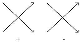

There exists different ways to describe a knot diagram: Planar Diagram, Gauss Code, Dowker Notation, Conway Notation.

Another way to describe a knot is to use quandles. From a knot K, we can construct the knot quandle Q(K), whose generators are the arcs of K, and relations are associated to the crossings: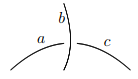

This figure gives us "a ▹ b = c" at a negative crossing, and "a ▹^-1 b = c" (or "c ▹ b = a") at a positive one.

gap> K:=PureCubicalKnot(3,1);;
gap> G:=GaussCodeOfPureCubicalKnot(K);;
gap> P:=PresentationKnotQuandle(G);
Quandle presentation of 3 generators and 3 relators.

gap> P!.generators;
[ 1 .. 3 ]
gap> P!.relators;
[ [ [ 3, 2 ], 1 ], [ [ 1, 3 ], 2 ], [ [ 2, 1 ], 3 ] ]

From this example, we see that the generators of the Trefoil Knot Quandle are the arcs 1, 2 and 3; these generators satisfy the relations above.

Nb: [[a₁ ,a₂ ],a₃ ] means a₁ ▹ a₂ = a₃, no matter if we consider a positive or negative crossing.

We can also easily go from a Planar Diagram representation of a knot to a its Gauss Code (with orientations of crossings).

gap> PD:=PlanarDiagramKnot(3,1);
[ [ 1, 4, 2, 5 ], [ 3, 6, 4, 1 ], [ 5, 2, 6, 3 ] ]
gap> G:=PD2GC(PD);
[ [ [ -1, 3, -2, 1, -3, 2 ] ], [ -1, -1, -1 ] ]

Using a finite connected quandle Q we can construct an invariant of a knot K: the number of homomorphisms Q_K---> Q from the fundamental quandle Q_K of K to the quandle Q.

gap> QK:=PresentationKnotQuandleKnot(12,1000);
Quandle presentation of 12 generators and 12 relators.

gap> Q:=ConnectedQuandle(30,2);;

gap> NumberOfHomomorphisms(QK,Q);
1230

For the same knot K (knot 1000 in the list of 12 crossing prime knots) we can compute the knot group W, the inner automorphism group RQ of the connected quandle Q of order 30, and the number of group homomorphisms W ---> RQ. This number is also an invariant of the knot.

gap> RQ:=RightMultiplicationGroupOfQuandleAsPerm(Q);;
gap> Order(RQ);
600
gap> PD:=PlanarDiagramKnot(12,1000);;
gap> G:=PD2GC(PD);;
gap> W:=SimplifiedFpGroup(WirtingerGroup(G));;
gap> NumberOfHomomorphisms(W,RQ);
13200

The following code shows how a partition of the number of homomorphisms K--->Q from a knot quandle K to a finite quandle Q can be used to distinguish between knots. The code establishes that by using only connected quandles Q of order ≤13, one can distinguish between all prime knots on at most eight crossings.

gap> L:=[];;
gap> for n in [1..8] do
> for i in [1..NumberOfPrimeKnots(n)] do
> Add(L,PresentationKnotQuandleKnot(n,i));
> od; od;

gap> inv:=function(K,n);
> return List(ConnectedQuandles(n),x->PartitionedNumberOfHomomorphisms(K,x));
> end;;

gap> C:=Classify(L,K->inv(K,3));; List(C,Size);
[ 11, 23, 1 ]
gap> C4:=RefineClassification(C,K->inv(K,4));; List(C4,Size);
[ 8, 3, 6, 17, 1 ]
gap> C5:=RefineClassification(C4,K->inv(K,5));; List(C5,Size);
[ 5, 2, 1, 1, 1, 1, 1, 1, 4, 3, 12, 1, 1, 1 ]
gap> C6:=RefineClassification(C5,K->inv(K,5));; List(C6,Size);
[ 1, 4, 1, 1, 1, 1, 1, 1, 1, 1, 4, 3, 12, 1, 1, 1 ]
gap> C7:=RefineClassification(C6,K->inv(K,7));; List(C7,Size);
[ 1, 1, 3, 1, 1, 1, 1, 1, 1, 1, 1, 4, 1, 1, 1, 2, 8, 2, 1, 1, 1 ]
gap> C8:=RefineClassification(C7,K->inv(K,8));; List(C8,Size);
[ 1, 1, 3, 1, 1, 1, 1, 1, 1, 1, 1, 4, 1, 1, 1, 1, 1, 6, 2, 2, 1, 1, 1 ]
gap> C9:=RefineClassification(C8,K->inv(K,9));; List(C9,Size);
[ 1, 1, 1, 1, 1, 1, 1, 1, 1, 1, 1, 1, 1, 1, 3, 1, 1, 1, 1, 1, 1, 3, 2, 1, 1, 1, 1, 1, 1, 1 ]
gap> C10:=RefineClassification(C9,K->inv(K,10));; List(C10,Size);
[ 1, 1, 1, 1, 1, 1, 1, 1, 1, 1, 1, 1, 1, 1, 3, 1, 1, 1, 1, 1, 1, 3, 2, 1, 1, 1, 1, 1, 1, 1 ]
gap> C11:=RefineClassification(C10,K->inv(K,11));; List(C11,Size);
[ 1, 1, 1, 1, 1, 1, 1, 1, 1, 1, 1, 1, 1, 1, 2, 1, 1, 1, 1, 1, 1, 1, 2, 1, 1, 1, 1, 1, 1, 1, 1, 1, 1 ]
gap> C12:=RefineClassification(C11,K->inv(K,12));; List(C12,Size);
[ 1, 1, 1, 1, 1, 1, 1, 1, 1, 1, 1, 1, 1, 1, 2, 1, 1, 1, 1, 1, 1, 1, 1, 1, 1, 1, 1, 1, 1, 1, 1, 1, 1, 1 ]
gap> C13:=RefineClassification(C12,K->inv(K,13));; List(C13,Size);
[ 1, 1, 1, 1, 1, 1, 1, 1, 1, 1, 1, 1, 1, 1, 1, 1, 1, 1, 1, 1, 1, 1, 1, 1, 1, 1, 1, 1, 1, 1, 1, 1, 1, 1, 1 ]

Given a quandle Q one defines the adjoint group Adj(Q) to be the group with one generator for each element of Q and relators

x^-1yx= x▹y

for x,y ∈ Q.

Q:=ConnectedQuandle(7,1);
<magma with 7 generators>

gap> F:=AdjointGroupOfQuandle(Q);
<fp group on the generators [ f1, f2, f3, f4, f5, f6, f7 ]>

The set of path components of a quandle Q is defined to be the set of orbits of the action of the right multiplication group Inn(Q) on Q. One can readily see that the rank of the abelianization of Adj(Q) is equal to the number of path components. The following code illustrates this.

gap> Q:=ConjugationQuandle(SymmetricGroup(5),1);
<magma with 10 generators>

gap> F:=AdjointGroupOfQuandle(Q);
<fp group with 120 generators>

gap> AbelianInvariants(F);
[ 0, 0, 0, 0, 0, 0, 0 ]

gap> P:=PathComponents(Q);;
gap> Size(P);
7

For a connected quandle Q the group A=Adj(Q) is isomorphic to a semi-direct product A=Z ⋊ D where D is the derived subgroup of Adj(Q) and Z is the infinite cylic group. There is a canonical group homomorphism Adj(Q) --> Inn(Q) to the right multiplication group. Thus Adj(Q) acts canonically on Q.

For a connected Q and preferred element q ∈ Q the fundamental group of Q at the base-point q is defined to be the subgroup of D consisting of those elements that fix q. Up to isomorphism the fundamental group of Q does not depend on the choice of base-point.

When Q is finite then so too is D. Thus for finite connected quandles one can compute the fundamental group directly from the definition.

gap> Q:=ConnectedQuandle(18,2);
<magma with 18 generators>

gap> F:=FundamentalGroup(Q);
<group with 2 generators>

gap> IdGroup(F);
[ 4, 1 ]

gap> D:=DerivedGroupOfQuandle(Q);
<group with 2 generators>

gap> IdGroup(D);
[ 72, 3 ]

A second example of a fundamental group computation is given below.

gap> Q:=ConjugationQuandle(SymmetricGroup(5),1);
<magma with 10 generators>

gap> P:=PathComponents(Q);;
gap> P:=List(P,x->AsMagma(x));;

gap> List(P,Size);
[ 1, 10, 20, 15, 30, 20, 24 ]

gap> List(P,IsConnected);
[ true, true, true, true, true, true, false ]

gap> Q:=P[5];
<magma with 3 generators>
gap> Size(Q);
30

gap> F:=FundamentalGroup(Q);
<group with 2 generators>

gap> IdGroup(F);
[ 4, 1 ]
gap>

Contents