| About HAP: Knots and Quandles |
Sub-package by Cédric FRAGNAUD and Graham ELLIS
1/ ∀∃∈For all a ∈ Q, a ▹ a = a.
2/ ∀ a, b ∈ Q, ∃! c ∈ Q such that a = c ▹ b.
3/ ∀ a, b, c ∈ Q, (a ▹ b) ▹ c = (a ▹ c) ▹ (b ▹ c).
One can check that for any group G and n ∈ ℤ, the magma (G, ▹) forms a quandle with the operation x ▹ y = y-nxyn , ∀ x, y ∈ G. Such a quandle is called the n-Fold Conjugation Quandle.
A quandle Q is said to be connected if the inner automorphism group Inn Q acts transitively on Q. In other words, Q is connected if and only if for each pair a, b in Q there are a1, a2, . . . , an in Q such that a ▹ a1 ▹· · · ▹ an = b.
A quandle Q is said to be latin if ∀ a, b ∈ Q, ∃ c ∈ Q such that a = b ▹ c.
<magma with 5 generators>
gap> Display(MultiplicationTable(Q));
[ [ 1, 3, 4, 5, 2 ],
[ 3, 2, 5, 1, 4 ],
[ 4, 5, 3, 2, 1 ],
[ 5, 1, 2, 4, 3 ],
[ 2, 4, 1, 3, 5 ] ]
gap> IsConnectedQuandle(Q);
true
gap> IsLatin(Q);
true
Then (Q,G,e,stigma) describes a Quandle Envelope if :
- G is a transitive group on Q.
- stigma ∈ Z(Ge), the center of the stabilizer of e.
- ⟨stigmaG⟩ = G (that is, the smallest normal subgroup of G containing stigma is all of G).
From a Quandle Envelope (Q,G,e,stigma), we can construct a Quandle (Q, ▹):
for all x,y in Q, x ▹ y=(ŷ(stigma))(x) , where ŷ ∈ G satisfies ŷ(e)=y.
Such a quandle is connected. This property is used to construct all the connected quandles of size n.
gap> IsQuandleEnvelope(Q,G,e,st); QE:=QuandleQuandleEnvelope(Q,G,e,st);
true
<magma with 9 generators>
gap> IsQuandle(QE); IsConnectedQuandle(QE);
true
true
gap> ConnectedQuandles(20); time;
[ <magma with 20 generators>, <magma with 20 generators>, <magma with 20 generators>,
<magma with 20 generators>, <magma with 20 generators>, <magma with 20 generators>,
<magma with 20 generators>, <magma with 20 generators>, <magma with 20 generators>,
<magma with 20 generators> ]
3364296
We define the right multiplication group G of a quandle Q by G=〈Rx, x ∈ Q〉.
We also define the automorphism group Aut(Q)={f:Q→Q}.
It can be proven that Rx is a subgroup of Aut(Q).
m6
gap> A:=AutomorphismGroupQuandle(Q);; a:=Random(A);;
gap> q^a;
m4
gap> R:=RightMultiplicationGroupOfQuandle(Q);; r:=Random(R);;
gap> q^r;
m3
To study these structures, we use knot diagrams, which are projections of these knots into ℝ2, defined, for instance, by f : ℝ3 → ℝ2; (x,y,z) → (x,y) subject to the constraint that the preimage of any (x, y) ∈ ℝ2 contains at most two points.
Crossing points occur when the preimage of a point in ℝ2 contains more than one point.
At these crossing points, we denote the point in the preimage that is nearer to the ℝ2 plane as the under-crossing point and the point farther away as the over-crossing point. An arc is a line that connects two crossing points in the knot diagram, with a line break occurring when an undercrossing point is mapped to the arc.
We may give a knot diagram an orientation, i.e. a direction of travelling around the knot. This allows us to categorize crossings as either positive or negative:

There exists different ways to describe a knot diagram: Planar Diagram, Gauss Code, Dowker Notation, Conway Notation.
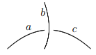
This figure gives us "a ▹ b = c" at a negative crossing, and "a ▹-1 b = c" (or "c ▹ b = a") at a positive one.
gap> G:=GaussCodeOfPureCubicalKnot(K);;
gap> P:=PresentationKnotQuandle(G);
rec( generators := [ 1 .. 3 ], relators := [ [ [ 3, 2 ], 1 ], [ [ 1, 3 ], 2 ], [ [ 2, 1 ], 3 ] ] )
Nb: [[a1 ,a2 ],a3 ] means a1 ▹ a2 = a3, no matter if we consider a positive or negative crossing.
[ [ 1, 4, 2, 5 ], [ 3, 6, 4, 1 ], [ 5, 2, 6, 3 ] ]
gap> G:=PD2GC(PD);
[ [ [ -1, 3, -2, 1, -3, 2 ] ], [ -1, -1, -1 ] ]
rec( generators := [ 1 .. 8 ], relators := [ [ [ 8, 2 ], 1 ], [ [ 2, 5 ], 1 ], [ [ 2, 6 ], 3 ], [ [ 3, 7 ], 4 ], [ [ 4, 8 ], 5 ],
[ [ 6, 1 ], 5 ], [ [ 6, 3 ], 7 ], [ [ 7, 4 ], 8 ] ] )
gap> Q:=ConnectedQuandle(9,2);;
gap> NumberHommorphism(Q,K); time;
9
216228
gap> Invariant(K,9); time;
[ 1, 3, 4, 5, 5, 5, 6, 6, 7, 7, 7, 7, 7, 64, 64, 8, 9, 9, 9, 9, 81, 9, 9, 9 ]
1327036
| Previous
Page |
Contents |
Next page |