| Previous |
About HAP: Knots, Links and Proteins |
next |
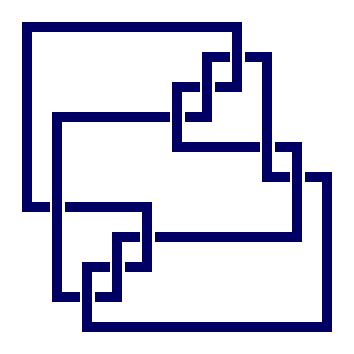
prime knot 10 with 9 crossings
gap> ViewPureCubicalKnot(K);
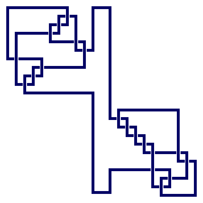
gap> L:=PureCubicalKnot(9,11);;
gap> M:=KnotSum(K,L);
prime knot 10 with 9 crossings + prime knot 11 with 9 crossings
gap> ViewPureCubicalKnot(M);
x_1^10-7*x_1^9+77/4*x_1^8-137/4*x_1^7+191/4*x_1^6-215/4*x_1^5+191/4*x_1^4-137/4*x_1^3+77/4*x_1^2-7*x_1+1
The following commands compute the abelian invariants of the low index subgroups of the knot group G (=fundamental group of knot complement) of the sum of the 10th and 11th knots on 9 crossings. The subgroups H<G of index at most 5 are computed. The abelian invariants are sorted so as to yield an isomorphism invariant of G.
We remark that the abelian invariants of subgroups of index at most 5 in the knot group are sufficient to distinguish between all prime knots on 9 or fewer crossings (up to ambient isotopy and mirror image).
gap> Invariants:=List(LowIndexSubgroupsFpGroup(G,5),AbelianInvariants);;
gap> Invariants:=SortedList(Invariants);
[ [ 0 ], [ 0, 0, 0 ], [ 0, 0, 0 ], [ 0, 0, 0 ], [ 0, 0, 0 ],
[ 0, 0, 0, 3, 3, 11, 11 ], [ 0, 0, 2, 3, 5, 7, 7 ], [ 0, 0, 2, 3, 5, 7, 7 ],
[ 0, 0, 2, 3, 5, 7, 7 ], [ 0, 0, 2, 3, 5, 7, 7 ],
[ 0, 0, 3, 3, 3, 7, 7, 11 ], [ 0, 0, 3, 11 ], [ 0, 0, 3, 11 ],
[ 0, 0, 3, 11, 11, 13, 13 ], [ 0, 2, 3, 3, 3, 3, 7, 7, 11 ],
[ 0, 2, 3, 3, 5, 7, 7, 8 ], [ 0, 2, 3, 3, 5, 7, 7, 8 ],
[ 0, 2, 3, 3, 5, 7, 7, 8 ], [ 0, 2, 3, 3, 5, 7, 7, 8 ],
[ 0, 2, 3, 3, 5, 11 ], [ 0, 3, 3, 3, 3, 11, 11 ], [ 0, 3, 3, 11, 11 ],
[ 0, 7, 7, 13, 13 ], [ 0, 59, 59, 79, 79 ] ]
gap> N:=PureCubicalKnot(C);
Pure cubical link.
gap> ViewPureCubicalKnot(N);

gap> G:=KnotGroup(N);
<fp group of size infinity on the generators [ f1, f2, f3 ]>
gap> RelatorsOfFpGroup(G);
[ f1*f2*f1^-1*f3*f2^-1*f3^-1, f2*f3^-1*f1^-1*f2*f3*f2^-1*f1^2*f2^-1*f1^-1 ]
<fp group of size infinity on the generators [ f1, f2, f3 ]>
gap> RelatorsOfFpGroup(G);
[ f1*f2*f1^-1*f3*f2^-1*f3^-1, f2*f3^-1*f1^-1*f2*f3*f2^-1*f1^2*f2^-1*f1^-1 ]
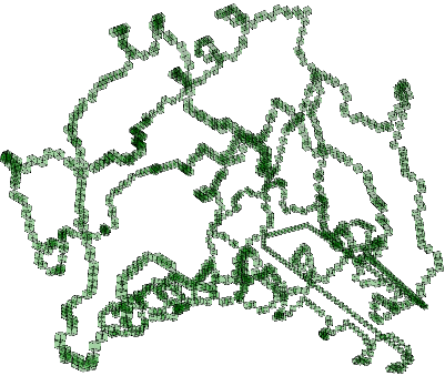
Read chain of 190 amino acids containing 1530 atoms.
Pure cubical complex of dimension 3.
gap> C:=ZigZagContractedPureCubicalComplex(C);;
gap> G:=FundamentalGroup(C);
<fp group of size infinity on the generators [ f1, f2 ]>
gap> RelatorsOfFpGroup(G);
[ f2*f1^-1*f2*f1*f2^-1*f1 ]
x_1^2-x_1+1
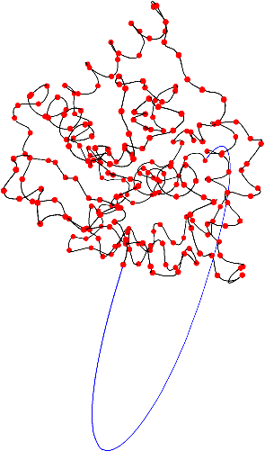
gap> Kprotein2:=ReadPDBfileAsPureCubicalComplex("1XD3.pdb",5);;
Reading chain containing 243 atoms.
gap> C:=ComplementOfPureCubicalComplex(Kprotein2);;
gap> C:=ZigZagContractedPureCubicalComplex(C);;
gap> G:=FundamentaGroup(C);;
#I there are 2 generators and 1 relator of total length 16
gap> AlexanderPolynomial(G);
x_1^2-3/2*x_1+1
gap> AlexanderPolynomial(PureCubicalKnot(5,2));
x_1^2-3/2*x_1+1
gap> ViewPureCubicalKnot(PureCubicalKnot(5,2));;

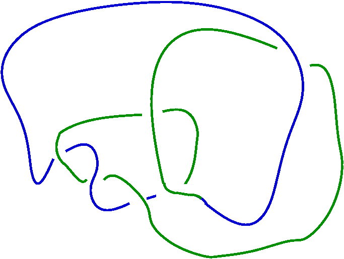
There may be slight errors in the coordinates of atoms in the pdb file for a protein. To test the robustness of the knottedness of a protein we can thicken the protein knot and see if its homotopy type changes. If the homotopy type does change then we can investigate whether the thickening has removed any knottedness.
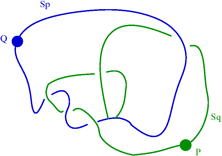
The following commands show that by thickening the Kprotein2 knot slightly we change its homotopy type to that of a wedge of two circles Sp v Sq, but that a further three thickenings contribute no further change of homotopy type.
gap> Kprotein2:=FramedPureCubicalComplex(Kprotein2);;
gap> Kprotein2:=FramedPureCubicalComplex(Kprotein2);; #This creates some space to perform thickenings
gap> T1:=ThickenedPureCubicalComplex(Kprotein2);;
gap> L:=ContractedComplex(T1);;
gap> Y:=CubicalComplexToRegularCWComplex(L);;
gap> CriticalCellsOfRegularCWComplex(Y);
[ [ 1, 571 ], [ 1, 601 ], [ 0, 6877 ] ]
gap> T2:=ThickenedPureCubicalComplex(T1);;
gap> T3:=ThickenedPureCubicalComplex(T2);;
gap> T4:=ThickenedPureCubicalComplex(T3);;
gap> L:=ContractedComplex(T4);;
gap> Y:=CubicalComplexToRegularCWComplex(L);;
gap> CriticalCellsOfRegularCWComplex(Y);
[ [ 1, 380 ], [ 1, 468 ], [ 0, 9436 ] ]
gap> C:=ZigZagContractedPureCubicalComplex(C);;
gap> Y:=CubicalComplexToRegularCWComplex(C);;
gap> CriticalCellsOfRegularCWComplex(Y);
[ [ 2, 68 ], [ 1, 88018 ], [ 1, 113335 ], [ 0, 49422 ] ]
gap> G:=FundamentalGroup(Y);
<fp group of size infinity on the generators [ f1, f2 ]>
gap> RelatorsOfFpGroup(G);
[ ]
gap> P:=ThickenedPureCubicalComplex(P);;
gap> P:=ThickenedPureCubicalComplex(P);;
gap> P:=ThickenedPureCubicalComplex(P);;
gap> P:=ThickenedPureCubicalComplex(P);;
gap> Sp:=PureCubicalComplexDifference(T3,P);;
gap> ContractPureCubicalComplex(Sp);;
gap> Sp:=ThickenedPureCubicalComplex(Sp);; #Makes Sp into a topology manifold again
gap> Cp:=ComplementOfPureCubicalComplex(Sp);;
gap> Cp:=ZigZagContractedPureCubicalComplex(Cp);;
gap> Yp:=CubicalComplexToRegularCWComplex(Cp);;
gap> CriticalCellsOfRegularCWComplex(Yp);
[ [ 1, 14 ], [ 0, 28 ] ]
gap> Q:=ThickenedPureCubicalComplex(Q);;
gap> Q:=ThickenedPureCubicalComplex(Q);;
gap> Q:=ThickenedPureCubicalComplex(Q);;
gap> Q:=ThickenedPureCubicalComplex(Q);;
gap> Sq:=PureCubicalComplexDifference(T3,Q);;
gap> ContractPureCubicalComplex(Sq);;
gap> Sq:=ThickenedPureCubicalComplex(Sq);; #Makes Sq into a topology manifold again
gap> Cq:=ComplementOfPureCubicalComplex(Sq);;
gap> Cq:=ZigZagContractedPureCubicalComplex(Cq);;
gap> Yq:=CubicalComplexToRegularCWComplex(Cq);;
gap> CriticalCellsOfRegularCWComplex(Yq);
[ [ 1, 27 ], [ 0, 19 ] ]
gap> Size(Sp);
2839
gap> ContractPureCubicalComplex(Sq);;
gap> Size(Sq);
747

and its complement.
However, a further three thickenings of the 1XD3 protein knot contribute no further changes to homotopy type.
| Previous
Page |
Contents |
Next
page |